

Bobby Durrett's DBA Blog
LLM Generates Summary of Detailed Report
DBAs spend a lot of time reviewing reports about the health of their databases. I’ve used an LLM to speed up that process.
I took a daily report about our Oracle databases and used an LLM to generate a short summary that lets a DBA immediately see which databases need attention.
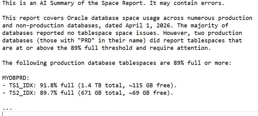
A typical report looks like this for each database:
The full report has over 2,000 lines that must be manually scanned by the on-call DBA each day.
The LLM-generated summary looks like this:
This summary immediately shows which databases need attention. We still manually scan the entire report but having the summary in the body of the email (with the full report attached) lets us see at a quick glance what needs attention and how urgent it is. The summary does not replace the full report; it only highlights the items that are most likely to be important. In our environment we chose 89% full as the point where we start reporting on space issues.
I’m using AWS Bedrock with the Claude Sonnet 4.6 model. Here is the Python
function that sends the combined prompt and report to Bedrock and returns the summary:
Here is the prompt that preceeds the report:
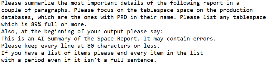
This simple use of an LLM has saved me time by putting a quick summary in the email body while preserving the full report for detailed review.
Bobby
ORA-04063 Errors During Datapatch Rollback of Oracle Patch 30763851
I am working on an Oracle 19c database running on a RHEL 7 VM. I have been trying to roll back this patch:
Patch 30763851 IMPDP 11.2 TO 18C OR HIGHER HITS ORA-904 WHEN TABLES HAVE EXTENDED STATISTICSI have it sitting on top of 19.5
Database Release Update: 19.5.0.0.191015 (30125133)The Opatch rollback command ran fine, but Datapatch threw these errors:
[2025-10-22 18:50:15]   -> Error at line 11329: script rdbms/admin/dpload.sql
[2025-10-22 18:50:15]       - ORA-04063: view "SYS.KU$_OPQTYPE_VIEW" has errors"
[2025-10-22 18:50:15]   -> Error at line 11331: script rdbms/admin/dpload.sql
[2025-10-22 18:50:15]       - ORA-04063: view "SYS.KU$_OPQTYPE_VIEW" has errors"
[2025-10-22 18:50:15]   -> Error at line 11333: script rdbms/admin/dpload.sql
[2025-10-22 18:50:15]       - ORA-04063: view "SYS.KU$_OPQTYPE_VIEW" has errors"
[2025-10-22 18:50:15]   -> Error at line 11335: script rdbms/admin/dpload.sql
[2025-10-22 18:50:15]       - ORA-04063: view "SYS.KU$_OPQTYPE_VIEW" has errors"
[2025-10-22 18:50:15]   -> Error at line 11337: script rdbms/admin/dpload.sql
[2025-10-22 18:50:15]       - ORA-04063: view "SYS.KU$_OPQTYPE_VIEW" has errors"
[2025-10-22 18:50:15]   -> Error at line 11339: script rdbms/admin/dpload.sql
[2025-10-22 18:50:15]       - ORA-04063: view "SYS.KU$_OPQTYPE_VIEW" has errors"
[2025-10-22 18:50:15]   -> Error at line 11341: script rdbms/admin/dpload.sql
[2025-10-22 18:50:15]       - ORA-04063: view "SYS.KU$_OPQTYPE_VIEW" has errors"
[2025-10-22 18:50:15]   -> Error at line 11343: script rdbms/admin/dpload.sql
[2025-10-22 18:50:15]       - ORA-04063: view "SYS.KU$_OPQTYPE_VIEW" has errors"
[2025-10-22 18:50:15]   -> Error at line 11355: script rdbms/admin/dpload.sql
[2025-10-22 18:50:15]       - ORA-04063: view "SYS.KU$_P2TPARTCOL_VIEW" has errors"
[2025-10-22 18:50:15]   -> Error at line 11357: script rdbms/admin/dpload.sql
[2025-10-22 18:50:15]       - ORA-04063: view "SYS.KU$_P2TPARTCOL_VIEW" has errors"
[2025-10-22 18:50:15]   -> Error at line 11363: script rdbms/admin/dpload.sql
[2025-10-22 18:50:15]       - ORA-04063: view "SYS.KU$_SP2TPARTCOL_VIEW" has errors"
[2025-10-22 18:50:15]   -> Error at line 11365: script rdbms/admin/dpload.sql
[2025-10-22 18:50:15]       - ORA-04063: view "SYS.KU$_SP2TPARTCOL_VIEW" has errors"
[2025-10-22 18:50:15]   -> Error at line 11381: script rdbms/admin/dpload.sql
[2025-10-22 18:50:15]       - ORA-04063: view "SYS.KU$_COLUMN_VIEW" has errors"
[2025-10-22 18:50:15]   -> Error at line 11383: script rdbms/admin/dpload.sql
[2025-10-22 18:50:15]       - ORA-04063: view "SYS.KU$_COLUMN_VIEW" has errors"
[2025-10-22 18:50:15]   -> Error at line 11385: script rdbms/admin/dpload.sql
[2025-10-22 18:50:15]       - ORA-04063: view "SYS.KU$_COLUMN_VIEW" has errors"
[2025-10-22 18:50:15]   -> Error at line 11387: script rdbms/admin/dpload.sql
[2025-10-22 18:50:15]       - ORA-04063: view "SYS.KU$_COLUMN_VIEW" has errors"
[2025-10-22 18:50:15]   -> Error at line 11389: script rdbms/admin/dpload.sql
[2025-10-22 18:50:15]       - ORA-04063: view "SYS.KU$_PCOLUMN_VIEW" has errors"
[2025-10-22 18:50:15]   -> Error at line 11391: script rdbms/admin/dpload.sql
[2025-10-22 18:50:15]       - ORA-04063: view "SYS.KU$_PCOLUMN_VIEW" has errors"
[2025-10-22 18:50:15]   -> Error at line 11393: script rdbms/admin/dpload.sql
[2025-10-22 18:50:15]       - ORA-04063: view "SYS.KU$_PCOLUMN_VIEW" has errors"
[2025-10-22 18:50:15]   -> Error at line 11395: script rdbms/admin/dpload.sql
[2025-10-22 18:50:15]       - ORA-04063: view "SYS.KU$_PCOLUMN_VIEW" has errors"
[2025-10-22 18:50:15]   -> Error at line 11397: script rdbms/admin/dpload.sql
[2025-10-22 18:50:15]       - ORA-04063: view "SYS.KU$_P2TCOLUMN_VIEW" has errors"
[2025-10-22 18:50:15]   -> Error at line 11399: script rdbms/admin/dpload.sql
[2025-10-22 18:50:15]       - ORA-04063: view "SYS.KU$_P2TCOLUMN_VIEW" has errors"
[2025-10-22 18:50:15]   -> Error at line 11401: script rdbms/admin/dpload.sql
[2025-10-22 18:50:15]       - ORA-04063: view "SYS.KU$_SP2TCOLUMN_VIEW" has errors"
[2025-10-22 18:50:15]   -> Error at line 11403: script rdbms/admin/dpload.sql
[2025-10-22 18:50:15]       - ORA-04063: view "SYS.KU$_SP2TCOLUMN_VIEW" has errors"
[2025-10-22 18:50:15]   -> Error at line 11405: script rdbms/admin/dpload.sql
[2025-10-22 18:50:15]       - ORA-04063: view "SYS.KU$_COLUMN_VIEW" has errors"
[2025-10-22 18:50:15]   -> Error at line 11407: script rdbms/admin/dpload.sql
[2025-10-22 18:50:15]       - ORA-04063: view "SYS.KU$_COLUMN_VIEW" has errors"
[2025-10-22 18:50:15]   -> Error at line 11409: script rdbms/admin/dpload.sql
[2025-10-22 18:50:15]       - ORA-04063: view "SYS.KU$_PCOLUMN_VIEW" has errors"
[2025-10-22 18:50:15]   -> Error at line 11411: script rdbms/admin/dpload.sql
[2025-10-22 18:50:15]       - ORA-04063: view "SYS.KU$_PCOLUMN_VIEW" has errors"
I checked DBA_OBJECTS, and all the SYS objects are VALID. I tried querying one of the views and it worked fine. So, I went to My Oracle Support, our Oracle database support site, and searched for ORA-04063 and one of the view names and found nothing. A Google search also came up empty. I tried just ignoring it but that didn’t work. My whole goal in doing this was to apply the October 2025 patches that just came out this week. But because the SQL patch registry indicated that patch 30763851 rolled back with errors, every time I applied a new patch it would try to roll 30763851 back first and error again. Here is what DBA_REGISTRY_SQLPATCH looked like after two failed rollback attempts:
INSTALL_ID   PATCH_ID PATCH_TYPE ACTION          STATUS
---------- ---------- ---------- --------------- --------------
         1   30125133 RU         APPLY           SUCCESS
         2   30763851 INTERIM    APPLY           SUCCESS
         3   30763851 INTERIM    ROLLBACK        WITH ERRORS
         3   30763851 INTERIM    ROLLBACK        WITH ERRORS
         4   30763851 INTERIM    ROLLBACK        WITH ERRORS
         4   30763851 INTERIM    ROLLBACK        WITH ERRORS
Each rollback attempt tried twice so I have four failures with two rollback attempts.
I opened a case with Oracle support just in case this was a known issue that wasn’t available for me to find on my own. Sometimes that happens. But while waiting on Oracle I kept trying to fix it myself.
The errors refer to $ORACLE_HOME/rdbms/admin/dpload.sql which I think reloads datapump after some change. It runs catmetviews.sql and catmetviews_mig.sql which have the CREATE VIEW statements for the views getting errors, like SYS.KU$_OPQTYPE_VIEW. But the code in catmetviews_mig.sql wasn’t straightforward. I imagined running some sort of trace to see why the script was throwing the ORA-04063 errors, but I never had to take it that far.
At first all this stressed me out. I thought, “I can’t back out this patch. I will never be able to patch this database to a current patch level.” Then I chilled out and realized that if it was a problem with Oracle’s code, they had to help me back out 30763851. But it might take some time to work through an SR with Oracle.
But what if it wasn’t an issue with Oracle’s code but something weird in our environment? I didn’t think it indicated a real problem, but there were some weird messages coming out that I am used to seeing. They were from triggers that come with an auditing tool called DB Protect. They were throwing messages like this:
[SYS.SENSOR_DDL_TRIGGER_A] Caught a standard exception: aliasId=100327, error=-29260, message="ORA-29260: network error: TNS:no listener"We are used to seeing these errors when we do DDL but prior to this it didn’t cause any actual problems. We had already decommisioned the DB Protect tool but had not cleaned up the triggers. Dropping SYS.SENSOR_DDL_TRIGGER_A eliminated the ORA-04063 errors.
Probably no one will ever encounter this same issue, but I thought I would document it. If you have the same symptoms and you are not using DB Protect any more, do these commands:
DROP TRIGGER SYS.SENSOR_DDL_TRIGGER_A;
DROP TRIGGER SYS.SENSOR_DDL_TRIGGER_B;
I think the A trigger was the problem, but we don’t need either one.
Anyway, this post is just so someone who searches for ORA-04063 and one of the views will find this information and drop the triggers if they have them. It’s a long shot but might as well document it for posterity and for me.
Bobby
Migrating WordPress to Amazon Linux 2023
I recently migrated my WordPress blog from Amazon Linux 2 to Amazon Linux 2023 to take advantage of newer software versions. The process was mostly smooth, but I wanted to document a few things I ran into—especially around encryption setup.
I followed these instructions for setting WordPress up on AL 2023: https://docs.aws.amazon.com/linux/al2023/ug/hosting-wordpress-aml-2023.html
The first thing I had to do was follow these instructions to get Apache, PHP, and MariaDB setup: https://docs.aws.amazon.com/linux/al2023/ug/ec2-lamp-amazon-linux-2023.html
I also had to setup a new elastic ip: https://docs.aws.amazon.com/AWSEC2/latest/UserGuide/elastic-ip-addresses-eip.html
I used the security group that I had for my existing AL 2 EC2 so I had the right ip addresses opened up.
I copied the database over from the old to new EC2:
on the old server:

mysqldump -u blogdbuser -pMYPASSWORD --single-transaction --routines --triggers blogdb  > blogdb.sql

on the new server:

mysql -vvv -n -u blogdbuser -pMYPASSWORD blogdb <  blogdb.sql > blogdb.log
Similarly for the web pages and other files:
New server:

# clear out existing web server directory

cd /var/www/html

sudo rm -fr *

sudo rm -f .htaccess .user.ini .wpcli

Old server:

sudo tar -cvf /home/ec2-user/html.tar /var/www/html

New server:

sudo tar -xvf /home/ec2-user/html.tar -C /
Moving the DNS entries over to the new elastic ip address was easy. I just had the change the “A” records for bobbydurrettdba.com and www.bobbydurrettdba.com in Route 53. First, I changed the TTL from one day to 10 minutes so my changes would propogate quickly while I messed with things. Later I set these back. One day was 86400 seconds. Ten minutes was 600 seconds.
The biggest challenge I had was getting encryption setup properly. The documentation missed a couple of key steps. I thought about just writing this post about the encryption part because it was the only thing that wasn’t straightforward.
I was following the steps in https://docs.aws.amazon.com/linux/al2023/ug/SSL-on-amazon-linux-2023.html and using the Let’s Encrypt script for getting certificates. This was called Certbot and documented here: https://eff-certbot.readthedocs.io/en/stable/install.html
There were two key things missing from this documentation:
- How to install Snap on Amazon Linux 2023
- The need for a port 80 VirtualHost
Certbot wants you to install something called Snap to use to install Certbot. I got this from a Google search:
sudo dnf install openssl mod_ssl

sudo wget -O /etc/yum.repos.d/snapd.repo https://bboozzoo.github.io/snapd-amazon-linux/al2023/snapd.repo

sudo dnf install snapd -y

sudo systemctl enable --now snapd.socket

sudo ln -s /var/lib/snapd/snap /snap

sudo reboot
The other undocumented thing was that I had to add these lines after the “Listen 80” line in /etc/httpd/conf/httpd.conf:
sudo vi /etc/httpd/conf/httpd.conf

after Listen 80 add this:

<VirtualHost *:80>
    DocumentRoot "/var/www/html"
    ServerName bobbydurrettdba.com
    ServerAlias www.bobbydurrettdba.com
</VirtualHost>
Then I just ran the documented Certbot commands like this:
sudo snap install --classic certbot

sudo ln -s /snap/bin/certbot /usr/bin/certbot

sudo certbot --apache
It took me a few iterations to get this right. Anyway, I just wanted to post a quick note documenting this.
Bobby
What I Learned About Machine Learning – Don’t Use It!
I set out to use Machine Learning to monitor Oracle databases but ultimately chose not to. The most valuable lesson I learned was the importance of visualizing my data to determine the best approach. By examining real production performance issues, I developed scripts that trigger alerts during potential performance problems. I used six weeks of historical performance metrics to compare current behavior against past trends. I already knew that a high value for a given metric didn’t necessarily indicate a performance issue with business impact. In the end, I built a script that sends an alert when certain metrics are the top wait event and are performing three times worse than at any point in the past six weeks. While it doesn’t guarantee a business impact, it flags anomalies that are unusual enough to warrant investigation.
2. Why I Tried Machine LearningI think anyone reading this post would know why I tried to use Machine Learning. It’s very popular now. I took a class online about ML with Python and I bought a book about the same subject. I had already used Python in some earlier classes and in my work, so it was natural to take a class/read a book about ML based on Python. As I mentioned in an earlier post, I studied AI in school many years ago and there have been many recent advances so naturally I wanted to catch up with the current state of the art in AI and ML. Having taken the class, and later having read a book, I needed some application of what I learned to a valuable business problem. We had a couple of bad performance problems with our Oracle databases and our current monitoring didn’t catch them. So, I wanted to use ML – specifically with PyTorch in a Python script – to write a script that would have alerted on those performance problems.
3. Failed Attempt Number One – AutoencoderIn my first attempt to write a monitoring script, I worked with Copilot and ChatGPT to hack together a script using an autoencoder model. I queried a bunch of our databases and collected a list of all the wait events. My idea was to treat each wait as an input to the autoencoder. For each wait, I pulled the number of events and the total wait time over the past hour. I didn’t differentiate between foreground and background waits—I figured AI could sort that out. I also included DB time and DB CPU time. These were all deltas between two hourly snapshots, so the data represented CPU and waits for a given hour.
The concept behind the autoencoder was to compress these inputs into a smaller set of values and then reconstruct the original inputs. With six weeks of hourly snapshots, I trained the autoencoder on that historical data, assuming it represented “normal” behavior. The idea was that any new snapshot that couldn’t be accurately reconstructed by the model would be considered abnormal and trigger an alert.
I got the model fully running across more than 20 production databases. I tuned the threshold so it would have caught two recent known performance issues. But in practice, it didn’t work well. It mostly triggered alerts on weekends when backups were running and I/O times naturally spiked. It wasn’t catching real performance problems—it was just reacting to predictable noise.
Here is the PyTorch autoencoder model:
# Define the Autoencoder model
class TabularAutoencoder(nn.Module):
    def __init__(self, input_dim):
        super(TabularAutoencoder, self).__init__()
        # Encoder
        self.encoder = nn.Sequential(
            nn.Linear(input_dim, 64),  # Reduce dimensionality from input_dim to 64
            #nn.LayerNorm(64),  # Layer Normalization for stability
            nn.ReLU(True),
            nn.Dropout(0.2),   # Dropout for regularization
            nn.Linear(64, 32),  # Reduce to 32 dimensions
            nn.ReLU(True),
            nn.Linear(32, 16),  # Bottleneck layer (compressing to 16 dimensions)
        )
        # Decoder
        self.decoder = nn.Sequential(
            nn.Linear(16, 32),  # Expand back to 32 dimensions
            nn.ReLU(True),
            nn.Linear(32, 64),  # Expand to 64 dimensions
            #nn.LayerNorm(64),  # Layer Normalization for stability
            nn.ReLU(True),
            nn.Linear(64, input_dim),  # Expand back to original input dimension
         )

    def forward(self, x):
        x = self.encoder(x)
        x = self.decoder(x)
return xMuch more recently, I came back to using a PyTorch model to build an alerting script. I had spent some time learning about large language models and exploring how to apply GenAI to business problems, rather than working with these simpler ML models in PyTorch. But I decided to give it another try and see if I could fix the limitations I ran into with the autoencoder approach.
I didn’t really expect binary classification to work, but it’s the simplest kind of ML model, so I thought it was worth a shot. I selected a few snapshots that occurred during a severe performance problem on an important Oracle database. I labeled these as 1 (problem), and the rest as 0 (no problem). It was easy enough to train a model that correctly identified the problem snapshots during training and testing.
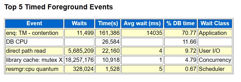
However, when I applied the model to later snapshots it hadn’t seen before, it started generating false alarms that didn’t make sense. It got even worse when I tried it on a completely different database. I had expected the model to pick up on the fact that the top wait event during the problem period was enq: TM – contention. A quick glance at the top foreground events in an AWR report made it obvious that this was the issue. But the trained model ended up sending an alert on snapshots that didn’t even have this wait event in the top waits.
Here is the PyTorch binary classification model:
"""

Mostly got the model from Copilot. input_dim is the number of performance
metrics which is over 100. Gets it down to 64 to 32 and then 1.
The ReLU functions add "non-linear" change to allow it to do
functions that the linear steps can't do.

"""

class MyModel(nn.Module):
    def __init__(self, input_dim):
        super(MyModel, self).__init__()
        self.fc1 = nn.Linear(input_dim, 64)
        self.relu1 = nn.ReLU()
        self.fc2 = nn.Linear(64, 32)
        self.relu2 = nn.ReLU()
        self.output = nn.Linear(32, 1)

    def forward(self, x):
        x = self.fc1(x)
        x = self.relu1(x)
        x = self.fc2(x)
        x = self.relu2(x)
        x = self.output(x)
        return x
Here are the foreground waits and cpu from an AWR report of the problem time:
 5. Failed Attempt Number Three – Z-Score
While talking with Copilot, I decided to try a simple statistical approach to anomaly detection. One suggestion was to use a z-score. In my context, this meant looking at the top foreground wait event—enq: TM – contention—in the current snapshot and calculating its z-score relative to the mean and standard deviation of that wait’s values in previous snapshots.
Like the binary classification attempt, the z-score alerting script worked well with the original snapshots from the known problem period. But when I ran the same script against other databases, it produced a lot of false alarms.
Output of z-score script on problem database (alerts on expected snapshot):
   SNAP_ID SNAP_DTTIME         EVENT_NAME            RATIO_ZSCORE AVGWAIT_ZSCORE
---------- ------------------- --------------------- ------------ --------------
    151752 2025-06-19 00:00:41 enq: TM - contention     3.0878532     9.74301378
Output on another database (no rows expected):
   SNAP_ID SNAP_DTTIME         EVENT_NAME                    RATIO_ZSCORE AVGWAIT_ZSCORE
---------- ------------------- ----------------------------- ------------ --------------
     48916 2025-06-22 01:00:01 cursor: pin S wait on X         9.00654128     5.36254393
     48917 2025-06-22 02:00:06 cursor: pin S wait on X         7.16211659     8.09929239
     48918 2025-06-22 03:00:11 cursor: pin S wait on X         5.41578347     4.52106805
     48919 2025-06-22 04:00:13 cursor: pin S wait on X         4.69593403     4.08335551
     48920 2025-06-22 05:00:16 cursor: pin S wait on X         3.17592316     3.46979661
     49081 2025-06-28 22:00:32 cursor: pin S wait on X         4.62636243     3.15122436
     49254 2025-07-06 03:00:04 cursor: pin S wait on X         4.73771834     3.23654318
     49255 2025-07-06 04:00:10 cursor: pin S wait on X         3.96208561     3.61732606
     49289 2025-07-07 14:00:55 SQL*Net more data from dblink   18.2249941     6.61795927
     49364 2025-07-10 17:00:20 library cache lock              89.7469665     392.322777
     49365 2025-07-10 18:00:45 library cache lock              14.6228987      120.71596
     49760 2025-07-27 05:00:21 cursor: pin S wait on X         5.68469758     3.52381292
Now I’m getting to the high point of this post. I graphed the waits for the snapshots where the z-score worked and the ones where it didn’t—and the truth jumped out at me. In the database with the known problem, the graph of enq: TM – contention was almost a flat line across the bottom for six weeks, followed by a huge spike during the problem hours. In another database—or even the same one with a different top wait—the graph looked completely different: a wavy pattern, almost like a sine wave, stretching back across the entire six weeks.
“Heck!” I said to myself. “Why don’t I just look for top waits that are never close to this high in the past six weeks?” Sure, it might not always be a real business problem, but if a wait is so dramatically different from six weeks of history, it’s worth at least sending an email—if not a wake-up-in-the-middle-of-the-night page.
With z-score, we were sending an alert when a metric was three standard deviations from the mean. But for wavy waits like db file sequential read, that wasn’t selective enough. So, I designed a new monitoring script: it looks at the top wait in the snapshot, checks if it’s a higher percentage of DB time than CPU, and then compares it to the past six weeks. If it’s more than three times higher than it’s ever been in that history, it triggers an alert. This is all based on the percentage of total DB time.
First the wavy graph of db file sequential read waits:
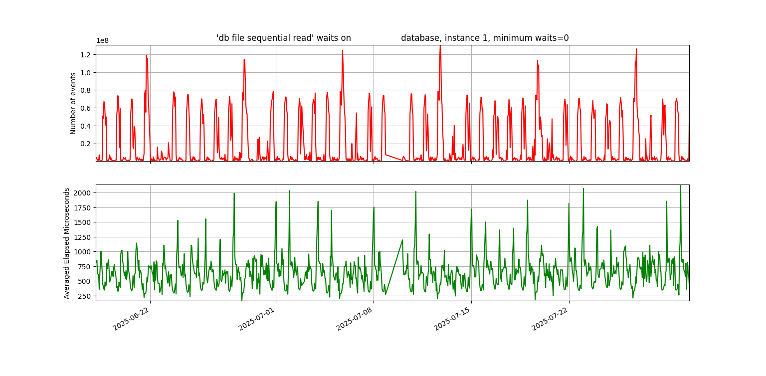
Next, this is the key graph to this entire post. Not wavy:
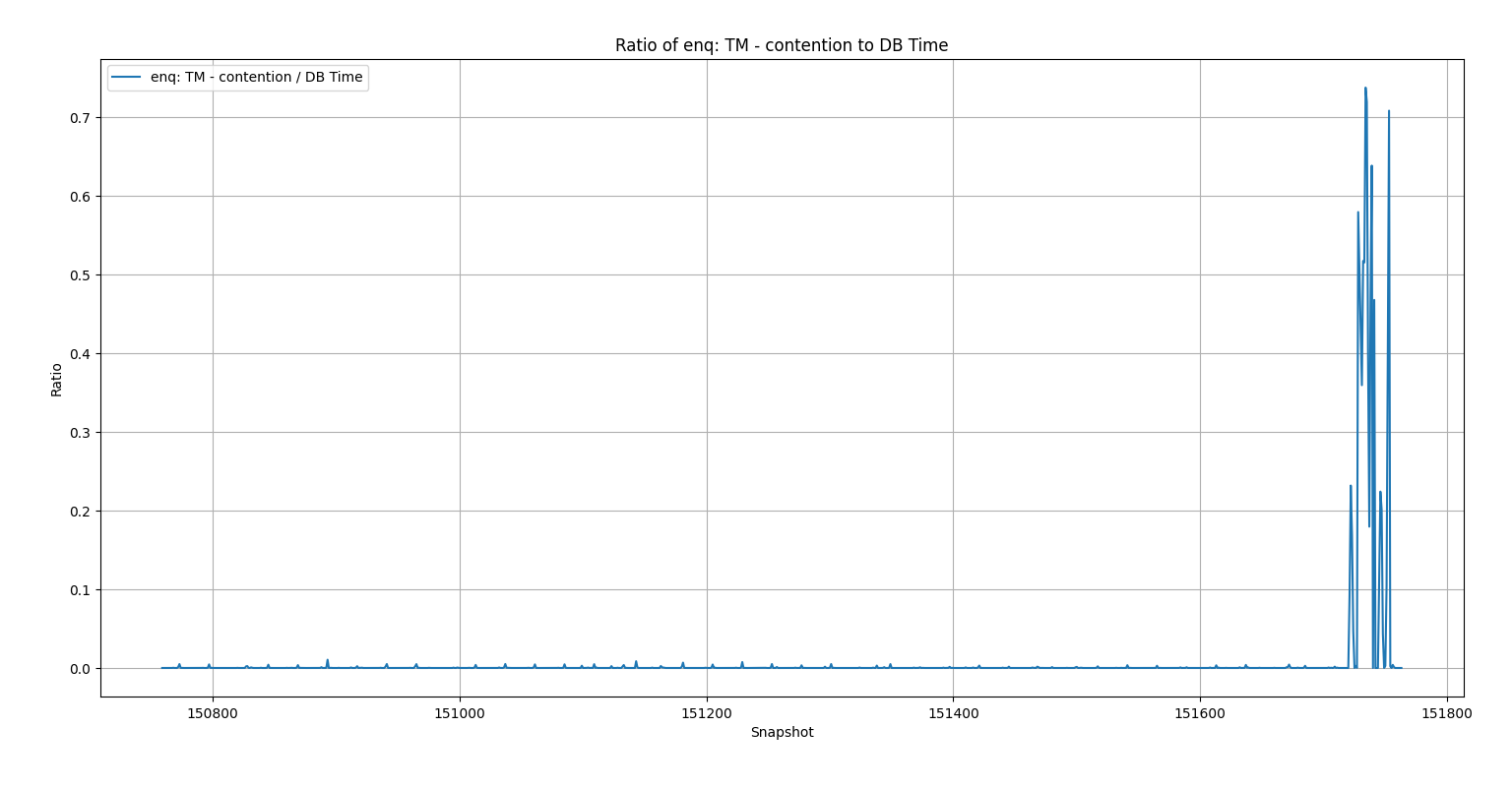
The light clicked on when I saw this graph. The enq: TM – contention waits were insignificant until the problem occurred.
Here is the script that checks if we should alert: neveralert.sql
7. Don’t Check Your Brain at the Machine Learning DoorWhen I started with the autoencoder script, I felt overwhelmed—like many people do when first approaching Artificial Intelligence and Machine Learning. I expected the model to magically work without fully understanding how or why. I relied on chat tools to help me piece together code I didn’t grasp, and when it didn’t work, I couldn’t explain why. I’m trying to be honest about my journey here so it might help others and remind myself what I learned.
Each step—from binary classification to z-score to manual logic—brought me closer to a solution rooted in my own experience. You must use your own brain. This has always been true in Oracle performance work: you can’t just follow something you read or heard about without understanding it. You need to think critically and apply your domain knowledge.
If it sounds like I didn’t get anything out of my machine learning training, that’s not the case. Both the class and the book emphasized the importance of visualizing data to guide modeling decisions. They used Matplotlib to create insightful graphs, and while I’ve used simpler visualizations in my own PythonDBAGraphs repo, this experience showed me the value of going deeper with data visualization. I think both the class and book would agree: visualizing your data is one of the best ways to decide how to use it.
Even though this journey didn’t end with a PyTorch-based ML solution, it sharpened my understanding of both ML and Oracle performance—and I’m confident it will help me build better solutions in the future.
Bobby
Picking Right Plan for SQL Profile
Sunday four batch jobs that normally run in an hour had been stuck for 3 hours and had not completed the first unit of work out of many. Earlier in the day the on call DBA had applied a SQL Profile and cancelled the jobs and rerun them but it did not help. We picked a different SQL Profile, killed the jobs, and the jobs ran normally. How did we figure out the right plan to use for a SQL Profile?
The main clue came from the output of my sqlstat.sql script:
The good plan seemed to be 2367956558. EXECUTIONS_DELTA = 1 means that the SQL finished in that hour. Elapsed Average ms of 45177.105 was 45 seconds. 19790.066 was 19 seconds.
PLAN_HASH_VALUE END_INTERVAL_TIME         EXECUTIONS_DELTA Elapsed Average ms
--------------- ------------------------- ---------------- ------------------
     2367956558 20-APR-25 01.00.23.638 AM                1          45177.105
     2367956558 20-APR-25 03.00.29.921 AM                1          19790.066
The other plans 2166514251 and 3151484146 seemed to have executions that spanned multiple hours. For example, the first 2166514251 line had EXECUTIONS_DELTA = 0 which means it didn’t finish in that hour. Plus, the elapsed time of 8995202.39 ms = 8995 seconds = 2.5 hours suggests that it was running in parallel, probably for the entire hour.
PLAN_HASH_VALUE END_INTERVAL_TIME         EXECUTIONS_DELTA Elapsed Average ms
--------------- ------------------------- ---------------- ------------------
     2166514251 20-APR-25 01.00.23.638 AM                0         8995202.39
So, it seems clear that 2367956558 is the best plan.
I could say a lot more about this incident, but I wanted to focus on the sqlstat.sql output. The values of EXECUTIONS_DELTA and Elapsed Average ms are keys to identifying plans with the best behavior.
Bobby
Matplotlib Oracle Example
Everyone who has heard the old saying “a picture is worth a thousand words” appreciates its simple wisdom. With Oracle databases you have situations where a graph of the output of a SQL query is easier to understand than the standard text output. It’s helpful to have a simple way to graph Oracle data, and Python has widely used libraries that make it easy.
This post describes a Python script that graphs data from an Oracle database using the Matplotlib graphics library. The script uses three widely used Python libraries: cx_Oracle, NumPy, and Matplotlib. This post provides a simple and easily understood example that can be reused whenever someone needs to graph Oracle data. It is written as a straight-line program without any functions or error handling to keep it as short and readable as possible. It demonstrates the pattern of cx_Oracle -> NumPy -> Matplotlib and the use of Matplotlib’s object-oriented approach.
Here is an example graph:
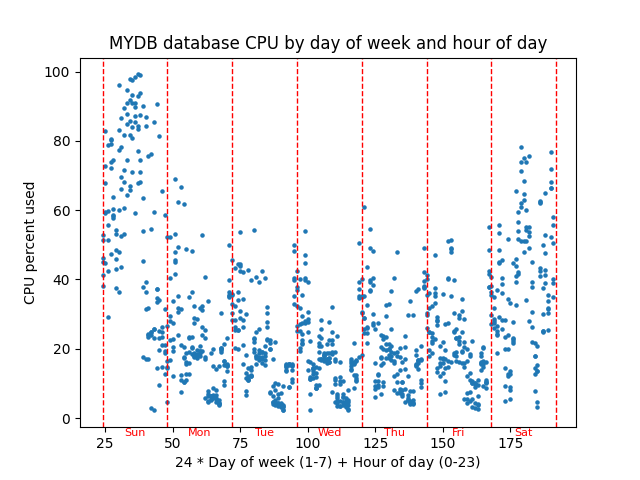
The script graphs database server percent CPU used versus a combination of the day of week and the hour of the day to see if there is any pattern of CPU usage throughout a typical week. This graph has about 6 weeks of hourly AWR snapshots graphed in a scatter plot with CPU percentage on the Y axis and (24 * day of week) + hour of day as the X axis. You could think of the X axis as the hour of the week. This graph might be helpful in performance tuning because it shows whether CPU usage follows a weekly pattern.
Here is the current version of the script: scatter.py.
The script has three main parts which correspond to the three non-internal Python libraries that I use:
- cx_Oracle – Query the CPU data from an Oracle database
- NumPy – Massage query data to get it ready to be graphed
- Matplotlib – Graph the data
These libraries all have lots of great documentation, but Matplotlib’s documentation is confusing at first. At least it was for me. Here are three useful links:
Quick start – This is a great overview. The picture of the “Parts of a Figure” is helpful. I don’t know if earlier versions of Matplotlib had this picture.
Axes – This is a nice list of all the methods of an Axes object. Most of the code in the example script involves calling these methods. I have trouble finding these methods using a Google search, so I bookmarked this link.
Figure – The example script does not call any Figure object methods, but I wanted to document where to find them here. I bookmarked this URL as well as the Axes one because a Matplotlib graph is composed of at least one Figure and Axes object. With the Quick start link and these two lists of methods you have all you need to write Matplotlib scripts.
cx_OracleThe query for this graph pulls operating system CPU metrics from the DBA_HIST_OSSTAT view and uses them to calculate the percent of the time the CPU is busy. It is made of two subqueries in a with statement and the final main query.
with
myoscpu as
(select
busy_v.SNAP_ID,
busy_v.VALUE BUSY_TIME,
idle_v.VALUE IDLE_TIME
from
DBA_HIST_OSSTAT busy_v,
DBA_HIST_OSSTAT idle_v
where
busy_v.SNAP_ID = idle_v.SNAP_ID AND
busy_v.DBID = idle_v.DBID AND
busy_v.INSTANCE_NUMBER = idle_v.INSTANCE_NUMBER AND
busy_v.STAT_NAME = 'BUSY_TIME' AND
idle_v.STAT_NAME = 'IDLE_TIME'),
The myoscpu subquery pulls the CPU busy and idle times from the view along with the snapshot id. I think these are totals since the database last came up, so you have to take the difference between their values at two different points in time to get the CPU usage for that time.
myoscpudiff as
(select
after.SNAP_ID,
(after.BUSY_TIME - before.BUSY_TIME) BUSY_TIME,
(after.IDLE_TIME - before.IDLE_TIME) IDLE_TIME
from
myoscpu before,
myoscpu after
where before.SNAP_ID + 1 = after.SNAP_ID
order by before.SNAP_ID)
The myoscpudiff subquery gets the change in busy and idle time between two snapshots. It is built on myoscpu. My assumption is that the snapshots are an hour apart which is the case on the databases I work with.
select
to_number(to_char(sn.END_INTERVAL_TIME,'D')) day_of_week,
to_number(to_char(sn.END_INTERVAL_TIME,'HH24')) hour_of_day,
100*BUSY_TIME/(BUSY_TIME+IDLE_TIME) pct_busy
from
myoscpudiff my,
DBA_HIST_SNAPSHOT sn
where
my.SNAP_ID = sn.SNAP_ID
order by my.SNAP_ID
The final query builds on myoscpudiff to give you the day of the week which ranges from 1 to 7 which is Sunday to Saturday, the hour of the day which ranges from 0 to 23, and the cpu percent busy which ranges from 0 to 100.
import cx_Oracle
...
# run query retrieve all rows

connect_string = username+'/'+password+'@'+database
con = cx_Oracle.connect(connect_string)
cur = con.cursor()

cur.execute(query)

# returned is a list of tuples
# with int and float columns
# day of week,hour of day, and cpu percent

returned = cur.fetchall()
...
cur.close()
con.close()
The cx_Oracle calls are simple database functions. You connect to the database, get a cursor, execute the query and then fetch all the returned rows. Lastly you close the cursor and connection.
print("Data type of returned rows and one row")
print(type(returned))
print(type(returned[0]))

print("Length of list and tuple")
print(len(returned))
print(len(returned[0]))

print("Data types of day of week, hour of day, and cpu percent")
print(type(returned[0][0]))
print(type(returned[0][1]))
print(type(returned[0][2]))
I put in these print statements to show what the data that is returned from fetchall() is like. I want to compare this later to NumPy’s version of the same data. Here is the output:
Data type of returned rows and one row
<class 'list'>
<class 'tuple'>
Length of list and tuple
1024
3
Data types of day of week, hour of day, and cpu percent
<class 'int'>
<class 'int'>
<class 'float'>
The data returned by fetchall() is a regular Python list and each element of that list is a standard Python tuple. The list is 1024 elements long because I have that many snapshots. I have 6 weeks of hourly snapshots. Should be about 6*7*24 = 1008. The tuples have three elements, and they are normal Python number types – int and float. So, cx_Oracle returns database data in standard Python data types – list, tuple, int, float.
So, we are done with cx_Oracle. We pulled in the database metric that we want to graph versus day and hour and now we need to get it ready to put into Matplotlib.
NumPyNumPy can do efficient manipulation of arrays of data. The main NumPy type, a ndarray, is a multi-dimensional array and there is a lot of things you can do with your data once it is in an ndarray. You could do the equivalent with Python lists and for loops but a NumPy ndarray is much faster with large amounts of data.
import numpy as np
...
# change into numpy array and switch columns
# and rows so there are three rows and many columns
# instead of many rows and three columns

dataarray = np.array(returned).transpose()

# dataarray[0] is day of week
# dataarray[1] is hour of day
# dataarray[2] is cpu percent
The function np.array() converts the list of tuples into a ndarray. The function transpose() switches the rows and columns so we now have 3 rows of data that are 1024 columns long whereas before we had 1024 list elements with size 3 tuples.
I added print statements to show the new types and numbers.
print("Shape of numpy array after converting returned data and transposing rows and columns")
print(dataarray.shape)

print("Data type of transposed and converted database data and of the first row of that data")
print(type(dataarray))
print(type(dataarray[0]))

print("Data type of the first element of each of the three transposed rows.")
print(type(dataarray[0][0]))
print(type(dataarray[1][0]))
print(type(dataarray[2][0]))
Here is its output:
Shape of numpy array after converting returned data and transposing rows and columns
(3, 1024)
Data type of transposed and converted database data and of the first row of that data
<class 'numpy.ndarray'>
<class 'numpy.ndarray'>
Data type of the first element of each of the three transposed rows.
<class 'numpy.float64'>
<class 'numpy.float64'>
<class 'numpy.float64'>
The shape of a ndarray shows the size of each of its dimensions. In this case it is 3 rows 1024 columns as I said. Note that the overall dataarray is a ndarray and any given row is also. So, list and tuple types are replaced by ndarray types. Also, NumPy has its own number types such as numpy.float64 instead of the built in int and float.
Now that our CPU data is in a NumPy array we can easly massage it to the form needed to plot points on our graph.
# do 24 * day of week + hour of day as x axis

xarray = (dataarray[0] * 24) + dataarray[1]

# pull cpu percentage into its own array

yarray = dataarray[2]
My idea for the graph is to combine the day of week and hour of day into the x axis by multiplying day of week by 24 and adding hour of the day to basically get the hours of the week from Sunday midnight to Saturday 11 pm or something like that. The nice thing about NumPy is that you can multiply 24 by the entire row of days of the week and add the entire row of hour of the day all in one statement. xarray is calculated in one line rather than writing a loop and it is done efficiently.
Here are some print statements and their output:
print("Shape of numpy x and y arrays")
print(xarray.shape)
print(yarray.shape)
Shape of numpy x and y arrays
(1024,)
(1024,)Now we have two length 1024 ndarrays representing the x and y values of the points that we want to plot.
So, we have used NumPy to get the data that we pulled from our Oracle database using cx_Oracle into a form that is ready to be graphed. Matplotlib works closely with NumPy and NumPy has some nice features for manipulating arrays of numbers.
MatplotlibNow we get to the main thing I want to talk about, which is Matplotlib. Hopefully this is a clean and straightforward example of its use.
import matplotlib.pyplot as plt
...
# get figure and axes

fig, ax = plt.subplots()
First step is to create a figure and axes. A figure is essentially the entire window, and an axes object is an x and y axis that you can graph on. You can have multiple axes on a figure, but for a simple graph like this, you have one figure, and one axes.
# point_size is size of points on the graph

point_size = 5.0
...
# graph the points setting them all to one size

ax.scatter(xarray, yarray, s=point_size)
This actually graphs the points. A scatter plot just puts a circle (or other shape) at the x and y coordinates in the two arrays. I set all points to a certain size and figured out what size circle would look best by trying different values. Note that scatter() is a method of the Axes type object ax.
# add title

ax.set_title(database+" database CPU by day of week and hour of day")

# label the x and y axes

ax.set_xlabel("24 * Day of week (1-7) + Hour of day (0-23)")
ax.set_ylabel("CPU percent used")
More methods on ax. Sets title on top center of graph. Puts labels that describe the x axis and the y axis.
# add vertical red lines for days

for day_of_week in range(8):
    ax.axvline(x=(day_of_week+1)*24, color='red', linestyle='--',linewidth=1.0)
The previous lines are all I really needed to make the graph. But then I thought about making it more readable. As I said before the X axis is basically the hour of the week ranging from 24 to 191. But I thought some red lines marking the beginning and end of each day would make it more readable. This puts 8 lines at locations 24, 48,…,192. I set the linewidth to 1.0 and used the dashes line style to try to keep it from covering up the points. I think axvline means vertical line on Axes object.
# Calculate the y-coordinate for day names
# It should be a fraction of the range between the minimum and maximum Y values
# positioned below the lower bound of the graph.
# The minimum and maximum CPU varies depending on the load on the queried database.

lower_bound = ax.get_ylim()[0]
upper_bound = ax.get_ylim()[1]
yrange = upper_bound - lower_bound
fraction = .025
y_coord = lower_bound - (fraction * yrange)

xloc = 36

for day in ['Sun','Mon','Tue','Wed','Thu','Fri','Sat']:
    ax.text(xloc, y_coord, day, fontsize=8, color='red', ha='center',fontweight='ultralight')
    xloc += 24
I kept messing with the script to try to make it better. I didn’t want to make it too complicated because I wanted to use it as an example in a blog post. But then again, this code shows some of the kinds of details that you can get into. The text() method of ax just puts some text on the graph. I made it red like the dashed lines and tried to make the letters light so they wouldn’t obscure the main parts of the graph. The x coordinates were just the center of the word and essentially the middle of the day. The first day starts at x=24 so 12 hours later or x=36 would be halfway through the day, approximately. I just had a list of the three-character day names and looped through them bumping the x location up by 24 hours for each day.
But the y coordinate was more complicated. I started out just choosing a fixed location for y like -5. For one database this worked fine. Then I tried another database, and it was way off. The reason is that Matplotlib scales the y coordinates based on the graphed data. If your database’s cpu is always around 30% then the range of visible y coordinates will be close to that. If your database’s cpu varies widely from 0% to 100% then Matplotlib will set the scale wide enough so the entire range 0 to 100 is visible. So, to put the text where I wanted it, just below the y axis line, I needed to make it a percentage of the visible y range below the lowest visible value. The get_ylim() method shows the calculated lower and upper bounds of the y axis which were calculated based on the y values of the graphed points. I manually messed with the value for the variable fraction until it looked right on the screen. Then I ran the script with a variety of databases to make sure it looked right on all of them.
# show graph

plt.show()
Lastly you just show the graph. Note that like the subplots() call this is not a method of an axes or figure object but just a matplotlib.pyplot call. Everything else in this example is a call to a method of the ax Axes type object.
ConclusionThis post shows how to graph Oracle database data using Python libraries cx_Oracle, NumPy, and Matplotlib. It first shows how to pull Oracle data into Python’s native data structures like lists and tuples. Then it shows how to convert the data into NumPy’s ndarrays and manipulate the data so that it can be graphed. Lastly it shows how to use Matplotlib Axes object methods to graph the data and add useful elements to the graph such as labels, vertical lines, and text.
This is a simple example, and all the software involved is free, open-source, widely used, easy to install, and well-documented. Give it a try!
2025 Update
I am not a very good blogger. Only four posts in 2024. I will need to pick it up because I just increased my spend on AWS for this blog. This site kept going down and I finally spent a few minutes looking at it and found that it was running out of memory. I was running on a minimal t2.micro EC2 which has 1 virtual CPU and 1 gigabyte of memory with no swap. So, rather than just add swap I bumped it up to a t3.small and paid for a 3-year reserved instance. It was about $220, nothing outrageous. Worth it to me. I still have two years left on the t2.micro reserved instance that I was using for the blog so I need to find a use for it, but I don’t regret upgrading. I spent a little money to make the site more capable so now I must write more posts!
I have three Machine Learning books to work through. After finishing my edX ML class with Python I picked up a book that covered the same topics and used the same Python libraries and I have been steadily working through it: Machine Learning with PyTorch and Scikit-Learn. I am on chapter 9 and want to get up to chapter 16 which covers Transformers. My edX class got up to the material in chapter 15 so the book would add to what was taught in the class. Earlier chapters also expand on what was taught in the class. The cool thing about the book is the included code. Lots of nice code examples to refer to later. Even the Matplotlib code for the graphs could be very helpful to me. I’ve gotten away from using Matplotlib after using it in my PythonDBAGraphs scripts.
My birthday is the day after Christmas, so I get all my presents for the year at the end of December. I got two ML books for Christmas/Birthday. Probably the first I will dive into after I finish the PyTorch/Scikit-Learn book is Natural Language Processing with Python. This is available for free on the NLTK web site. I have the original printed book. I think once I get through the Transformers chapter of the PyTorch book it makes sense to look at natural language processing since that is what ChatGPT and such is all about. I have played with some of this already, but I like the idea of working through these books.
The second book that I got in December as a present seems more technical and math related, although the author claims to have kept the math to a minimum. It is Pattern Recognition and Machine-Learning. This might be a slower read. It seems to be available for free as a PDF. ChatGPT recommended this and the NLTK book when I was chatting with it about my desire to learn more about Artificial Intelligence and Machine Learning.
I have all these conversations with ChatGPT about whether it makes sense for me as an Oracle database specialist to learn about machine learning. It assures me that I should, but it might be biased in favor of ML. Oracle 23ai does have AI in its name and does have some machine learning features. But it could just be a fad that blows over after the AI bubble bursts as many have before it. I can’t predict that. My current job title is “Technical Architect”. I work on a DBA team and I’m in the on-call rotation like everyone else, but my role includes learning about new technology. Plus, I think that I personally add value because of some of the computer science background I had in school and that I have been refreshing in recent years. Plus, I need to get some level of understanding of machine learning for my own understanding regardless of how much we do or don’t use it for my job. Just being a citizen of the world with a computer science orientation I feel is enough motivation to get up to speed on recent AI advancements. Am I misguided to think I should study machine learning?
Despite all this talk about AI, I am still interested in databases. I have this folder on my laptop called “Limits of SQL Optimization”. I had these grandiose ideas about writing interesting blog posts about what SQL could or couldn’t do without human intervention. Maybe SQL is a little like AI because the optimizer does what a human programmer would have to do without it. I’m interested in it all really. I like learning about how computer things work. I’ve spent my career so far working with SQL statements and trying to understand how the database system processes them. I thought about playing with MySQL’s source code. I downloaded it and compiled it but that’s about it. Plus, some day we will have Oracle 23ai and I’ll have to figure out how to support it in our environment, even if we do not use its AI features. Anyway, I’m sure I will have some non-AI database things to post about here.
To wrap up I think I may have some things to post on this blog in 2025, so it’s worth the extra expense to keep it running. Could be some more machine learning/artificial intelligence coming as I work through my books. I still have databases on the brain. Wish you all a great new year.
Bobby
Using PyTorch to Predict Host CPU from Date/Time
In my previous post I mentioned that I took a machine learning class based on Python and a library called PyTorch. Since the class ended, I have been working on a useful application of the PyTorch library and machine learning ideas to my work with Oracle databases. I do not have a fully baked script to share today but I wanted to show some things I am exploring about the relationship between the current date and time and database performance metrics such as host CPU utilization percentage. I have an example that you can download here: datetimeml2.zip
There is a relationship between the day of the week and the hour of the day and database performance metrics on many Oracle database systems. This is a graph from my hostcpu.py script that shows CPU utilization on a production Oracle database by date and hour of the day:
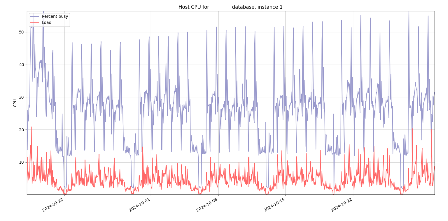
During the weekdays the CPU peaks at a certain hour and on the weekends, there are some valleys. So, I thought I would use PyTorch to model this relationship. Here is what the graph looks like of actual host CPU used versus predicted by PyTorch:
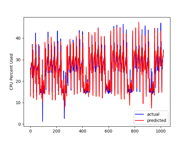
It’s the same source database but an earlier date. The prediction is close. I guess the big question after I got to this point was, so what? I’m not sure exactly what to do with it now that I have a model of the database CPU. I guess if the CPU is at 100% for an entire day instead of going up and down, I should throw an alert? What if CPU stays near 0% for a day during the week? It must be helpful to have a prediction of the host CPU but exactly how to alert on deviations from the predicted value is still a work in progress.
I thought it would be helpful to talk about the date and time inputs to this model. If you look at datetimeoscpu.sql in the zip it has this SQL for getting the date and time values:
select
to_char(sn.END_INTERVAL_TIME,'D') day_of_week,
to_char(sn.END_INTERVAL_TIME,'DD') day_of_month,
to_char(sn.END_INTERVAL_TIME,'DDD') day_of_year,
to_char(sn.END_INTERVAL_TIME,'HH24') hour_of_day,
to_char(sn.END_INTERVAL_TIME,'MM') month,
to_char(sn.END_INTERVAL_TIME,'Q') quarter,
to_char(sn.END_INTERVAL_TIME,'WW') week_of_year,
to_char(sn.END_INTERVAL_TIME,'W') week_of_month,
to_char(sn.END_INTERVAL_TIME,'YYYY') year,
...
I ended up ignoring year because it is not a cyclical value. The rest have a range like 1 to 7 for day of week or 1 to 31 for day of month. Having all eight of these is probably overkill. I could just focus on day of week and hour of day and forget the other six. We have 6 weeks of AWR history so I’m not sure why I care about things like month, quarter, day of year because I don’t have multiple years of history to find a pattern.
My input data looks like this:
4 17 199 03 07 3 29 3 2024            15.4210261
4 17 199 04 07 3 29 3 2024            15.5799532
4 17 199 05 07 3 29 3 2024            26.2080227
4 17 199 06 07 3 29 3 2024            24.1532019
4 17 199 07 07 3 29 3 2024            23.2947767
4 17 199 08 07 3 29 3 2024            25.5198717
4 17 199 09 07 3 29 3 2024             26.029638
4 17 199 10 07 3 29 3 2024            27.1160204
4 17 199 11 07 3 29 3 2024            27.7076496
Each line represents an AWR snapshot. The first 8 are the cyclical date and time input values or X. The last value is the host CPU utilization percentage or Y. The point of the program is to create a model based on this data that will take in the 8 values and put out a predicted CPU percentage. This code was used to make the predictions for the graph at the end of the train.py script:
predictions = model(new_X)When I first started working on this script it was not working well at all. I talked with ChatGPT about it and discovered that cyclical values like hour of day would work better with a PyTorch model if they were run through sine and cosine to transform them into the range -1 to 1. Otherwise PyTorch thinks that an hour like 23 is far apart from the hour 0 when really, they are adjacent. Evidently if you have both cosine and sine their different phases help the model use the cyclical date and time values. So, here is the code of the function which does sine and cosine:
def sinecosineone(dttmval,period):
    """
    Use both sine and cosine for each of the periodic
    date and time values like hour of day or
    day of month

    """
    # Convert dttmval to radians
    radians = (2 * np.pi * dttmval) / period
    # Apply sine and cosine transformations
    sin_dttmval = np.sin(radians)
    cos_dttmval = np.cos(radians)
    return sin_dttmval, cos_dttmval

def sinecosineall(X):
    """
    Column         Number

    day_of_week      7
    day_of_month     31
    day_of_year      366
    hour_of_day      24
    month            12
    quarter          4
    week_of_year     52
    week_of_month    5

    """
...
The period is how many are in the range – 24 for hour of the day. Here is the hour 23 and hour 0 example:
>>> sinecosineone(23.0,24.0)
(-0.25881904510252157, 0.9659258262890681)
>>> sinecosineone(0.0,24.0)
(0.0, 1.0)
Notice how the two values are close together for the two hours that are close in time. After running all my input data through these sine and cosine procedures they are all in the range -1.0 to 1.0 and these were fed into the model during training. Once I switched to this method of transforming the data the model suddenly became much better at predicting the CPU.
You can play with the scripts in the zip. I really hacked the Python script together based on code from ChatGPT, and I think one function from my class. It isn’t pretty. But you are welcome to it.
I’m starting to get excited about PyTorch. There are a bunch of things you must learn initially but the fundamental point seems simple. You start with a bunch of existing data and train a model that can be used as a function that maps the inputs to the outputs just as they were in the original data. This post was about an example of inputting cyclical date and time values like time of day or day of week and outputting performance metrics like CPU used percentage. I don’t have a perfect script that I have used to great results in production, but I am impressed by PyTorch’s ability to predict database server host CPU percent based on date and time values. More posts to come, but I thought I would get this out there even though it is imperfect. I hope that it is helpful.
Bobby
Catching Myself up on AI: Useful Resources
In this post, I will describe the AI training resources that I am using in my quest to catch up with the current state of the art. My goal is to document the resources that I used for my own reference and to benefit others while explaining my reasoning along the way.
After studying AI back in the 1980s, I have not kept my AI skills up to date until recently when I started learning about newer things like ChatGPT. AI is in the news and every technical person should learn something about it for their own understanding and to help their career. Because I had a good overall understanding of the state of AI years ago, I think of it as “catching up” with the present-day standard. So, my approach makes sense for me given my history. But even for people who are not as old as I am or who don’t have the AI experience from their past the resources below could still be useful because of their overall quality.
Revisit AI Overview – 6.034The first thing I did was watch the lecture videos for Patrick Winston‘s 2010 MIT 6.034 class. I had used Winston’s textbook in my college AI class in the 1980s. So, I thought that a class taught my Winston might follow a similar outline to what I once knew about AI and help jog my memory and catch me up with what has changed in the last 30+ years. Just watching the lecture videos and not doing the homework and reading limited how much I got from the class, but it was a great high-level overview of the different areas of AI. Also, since it was from 2010 it was good for me because it was closer to present day than my 1980s education, but 14 years away from the current ChatGPT hoopla. One very insightful part of the lecture videos is lectures 12A and 12B which are about neural nets and deep neural nets. Evidently in 2010 Professor Winston said that neural nets were not that promising or could not do that much. Fast forward 5 years and he revised that lecture with two more modern views on neural nets. Of course, ChatGPT is based on neural nets as are many other useful AI things today. After reviewing the 6.034 lecture videos I was on the lookout for a more in depth, hands on, class as the next step in my journey.
edX Class With Python – 6.86xI had talked with ChatGPT about where to go next in my AI journey and it made various suggestions including books and web sites. I also searched around using Google. Then I noticed an edX class about AI called “Machine Learning with Python-From Linear Models to Deep Learning,” or “6.86x”. I was excited when I saw that edX had a useful Python-based AI class. I had a great time with the two earlier Python edX classes which I took in 2015. They were:
- 6.00.1x – Introduction to Computer Science and Programming Using Python
- 6.00.2x – Introduction to Computational Thinking and Data Science
This blog has several posts about how I used the material in those classes for my work. I have written many Python scripts to support my Oracle database work including my PythonDBAGraphs scripts for graphing Oracle performance metrics. I have gotten a lot of value from learning Python and libraries like Matplotlib in those free edX classes. So, when I saw this machine learning class with Python, I jumped at the chance to join it with the hope that it would have hands-on Python programming with libraries that I could use in my regular work just as the 2015 classes had.
Math PrerequisitesI almost didn’t take 6.86x because the prerequisites included vector calculus and linear algebra which are advanced areas of math. I may have taken these classes decades ago, but I haven’t used them since. I was afraid that I might be overwhelmed and not able to follow the class. But since I was auditing the class for free, I felt like I could “cheat” as much or as little as I wanted because the score in the class doesn’t count for anything. I used my favorite algebra system, Maxima, when it was too hard to do the math by hand. I had some very interesting conversations with ChatGPT about things I didn’t understand. My initial fears about the math were unfounded. The class helped you with the math as much as possible to make it easier to follow. And, at the end of the day since I wasn’t taking this class for any kind of credit, the points don’t matter. (like the Drew Carey improv show). What matters was that I got something out of it. I finished the class this weekend and although the math was hard at times I was able to get through it.
How to Finish Catching Up to 2024It looks like 6.86x is 4-5 years old so it caught me up to 2019. I have been thinking about where to go from here to get all the way to present day. Working on this class I found two useful Python resources that I want to pursue more:
- PyTorch – Neural Nets
- Hugging Face – Large Language Models
I walked away from both 6.034 and 6.86x realizing how important neural nets are to AI today and so I want to dig deeper into PyTorch which is a top Python library for neural nets originally developed by Facebook. With the importance of neural nets and the experience I got with PyTorch from the class it only makes sense to dig deeper into PyTorch as a tool that I can use in my database work. As I understand it Large Language Models such as those behind ChatGPT are built using tools like PyTorch. Plus, neural nets have many other applications outside of LLMs. I hope to find uses for PyTorch in my database work and post about them here.
Large Language Models with Hugging FaceEveryone is talking about ChatGPT and LLMs today. I ran across the Hugging Face site during my class. I can’t recall if the class used any of the models there or if I just ran across them as I was researching things. I would really like to download some of the models there and play with updating them and using them. I have played with LLM’s before but have not gotten very far. I tried out OpenAI’s API programming doing completions. I played with storing vectors in MongoDB. But I didn’t have the background that I have now from 6.86x to understand what I was working with. If I can find the time, I would like to both play with the models from Hugging Face and revisit my earlier experiments with OpenAI and MongoDB. Also, I think Oracle 23ai has vectors so I might try it out. But one thing at a time! First, I really want to dig into PyTorch and then mess with Hugging Face’s downloadable models.
RecapI introduced several resources for learning about artificial intelligence. MIT’s OCW class from 2010, 6.034, has lecture videos from a well-known AI pioneer. 6.86x is a full-blown online machine learning class with Python that you can audit for free or take for credit. Python library PyTorch provides cutting edge neural net functionality. Hugging Face lets you download a wide variety of large language models. These are some great resources to propel me on my way to catching up with the present-day state of the art in AI, and I hope that they will help others in their own pursuits of AI understanding.
Bobby
P.S. Here are a couple of fun screenshots from the last project in my 6.86x class. Hopefully it won’t give too much away to future students.
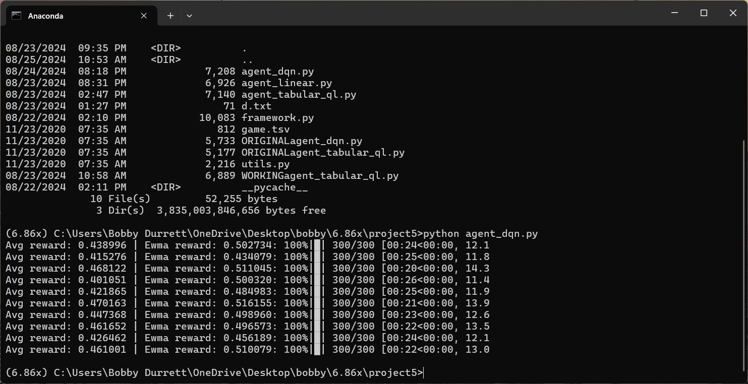
This is a typical run using PyTorch to train a model for the last assignment.
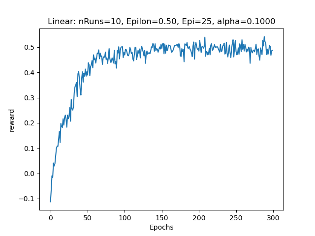
This is the graphical output showing when the training converged on the desired output.
Simple MySQL Range Scan Test
I was trying to tune a MySQL query this week. I ran the same query against Oracle with the same data and got a much faster runtime on Oracle. I couldn’t get MySQL to do a range scan on the column that Oracle was doing it on. So, I just started barely scratching the surface with a simple test of when MySQL will use an index versus a full table scan in a range query. In my test MySQL always uses an index except on extreme out of range conditions. This is funny because in my real problem query it was the opposite. But I might as well document what I found for what it’s worth. I haven’t blogged much lately.
Here is my testcase and its output:
https://www.bobbydurrettdba.com/uploads/mysqlindexuserangequeries.zip
This is on 8.0.26 as part of an AWS Aurora MySQL RDS instance with 2 cores and 16 gigabytes of RAM.
I created a simple test table and put 10485760 rows in it:
create table test
(a integer NOT NULL AUTO_INCREMENT,
b integer,
PRIMARY KEY (a));
The value of b is always 1 and a ranges from 1 to 10878873.
This query uses a range query using the index:
select
sum(b)
from
test
where
a > -2147483648;
This query uses a full table scan:
select
sum(b)
from
test
where
a > -2147483649;
The full scan is slightly faster.
Somehow when you are 2147483650 units away from the smallest value of a the MySQL optimizer suddenly thinks you need a full scan.
There are a million more tests I could do like things with a million variables, but I thought I might as well put this out there. I’m not really any the wiser but it is a type of test that might be worth mentioning.
Bobby
Archivelog Space Needed Python Script
I wrote a script called archivelogspace.py to help size our Oracle archive log filesystems to support replication tools such as Fivetran, DMS, or GoldenGate which need a certain number of hours or days of archive log history at all times. In many cases we had backups that removed all the archive logs after they had been backed up once. So, that is essentially zero hours of history. If we only backed up once per day, it really peaked out at 24 hours of history, but the minimum was zero. Our replication products need 24 hours minimum in some cases. In other cases, we needed different numbers of hours. Also, the log backups and deletes run multiple times a day and on different schedules on some systems.
I based archivelogspace.py on a simplistic idea which I know is not perfect but so far it has been helpful. So, I thought I would share it here in case others can benefit. I would love any feedback, suggestions and criticism of the approach and implementation. The idea was to query V$ARCHIVED_LOG and see how full the filesystem would get if these same logs came in at the same times but with different retention times and different archive log filesystem sizes. I could try different settings and see the highest percentage that the filesystem hit.
I think this approach is imperfect because the past behavior recorded in V$ARCHIVED_LOG may not represent future behavior very well as things change. Also, the way I wrote it I assumed that the archive logs are laid down instantaneously. I.e. If the row in V$ARCHIVED_LOG has COMPLETION_TIME of 2/24/2024 16:11:15 then I assume that the filesystem gets (BLOCKS+1)*BLOCK_SIZE bytes fuller in that second. I also assume that the backups instantly remove all the logs which are beyond the retention.
I tested the script using the current settings for the archive log filesystem size and log backup run times and retention settings. I just compared the output percent full with reality. It was close but not exact. So, when I went to apply this for real, I padded the filesystem sizes so the expected percent full was less than 50%. So far so good in reality. I would like to build an emergency script that automatically clears out old logs if the filesystem gets full but so far, I have not. We do have alerting on archive log filesystem space getting too full.
If you run the script, you can see the arguments:
Arguments: oracle-username oracle-password tns-name configfile-name

Config file is text file with this format:

archivelog filesystem size in bytes
number of backups per day
one line per backup with 24-hour:minutes:seconds archivlog-retention-hours

for example:

8795958804480
6
02:15:00 168
06:15:00 168
10:45:00 168
14:15:00 168
18:15:00 168
22:15:00 168
The output is something like this:
2024-02-20 08:55:57 1.67%
2024-02-20 09:10:02 1.68%
2024-02-20 10:00:29 1.69%
2024-02-20 11:00:20 1.7%
2024-02-20 11:37:32 1.7%
2024-02-20 12:01:17 1.68%
2024-02-20 12:09:05 1.68%
2024-02-20 12:43:53 1.69%
2024-02-20 12:55:52 1.69%

Max percent used archivelog filesystem: 46.15%
Date and time of max percent: 2023-12-24 11:52:17
When your archive log filesystem is too small the Max percent is over 100%.
It’s not perfect or fancy but it is available if someone finds it useful.
Bobby
p.s. The script uses cx_Oracle so you will need to install that.
User Privileges Script
I keep running into situations on Oracle databases where I need to dump out the privileges an Oracle user has. I have been just manually putting together SQL statements like:
select * from dba_role_privs where grantee='MYUSER';
select * from dba_sys_privs where grantee='MYUSER';
select * from dba_tab_privs where grantee='MYUSER';
select * from dba_users where username='MYUSER';
This captures the three kinds of grants the user could have in the first three queries and the last query just shows if the user exists and things like whether it is locked. Really this simple set of queries is good enough in most cases.
But I had also wrote a script that would show all the system and object grants that were included in the roles. Because you can have roles granted to roles, you must loop through all the roles until you get down to the base system and object privileges. I rewrote this logic from scratch several times until I finally convinced myself to make a script and save it on my GitHub site. The current version of the script is here:
The interesting part of the script is where we keep looping through the roles in table my_role_privs deleting each role and then inserting the role’s system, object, and role privileges into the my_sys_privs, my_tab_privs, and my_role_privs tables. Eventually you run out of roles to delete and the loop finishes. I guess this works because you cannot have a circular role grant situation:
SQL> create role a;

Role created.

SQL> create role b;

Role created.

SQL> grant a to b;

Grant succeeded.

SQL> grant b to a;
grant b to a
*
ERROR at line 1:
ORA-01934: circular role grant detected
In the past I have put a loop counter in the code just in case there was something circular or a really long chain of roles, but this version does not have it.
To make the output useful I put it in three sections. The first section just has the direct grants and corresponds to the first three queries listed above.
Privileges granted directly to user MYUSER

Role privileges for user MYUSER

GRANTED_ROLE
--------------------
DBA
RESOURCE

System privileges for user MYUSER

PRIVILEGE
----------------------------------------
SELECT ANY TABLE
UNLIMITED TABLESPACE

Summarized table privileges for user MYUSER

OWNER                PRIVILEGE                                  COUNT(*)
-------------------- ---------------------------------------- ----------
SYS                  EXECUTE                                           1

Detailed table privileges for user MYUSER

PRIVILEGE                                OWNER                TABLE_NAME
---------------------------------------- -------------------- -----------
EXECUTE                                  SYS                  DBMS_RANDOM
I put counts of each type of object grants in case there was a bunch. I called them table privileges because view is named dba_tab_privs but I really should have called them object privileges because they can be grants on objects which are not tables.
The second section has the output of the loop showing all the system and object privileges implied by the role grants as well as those granted directly to the user:
Privileges granted through a role or directly to user MYUSER

System privileges for user MYUSER

PRIVILEGE
----------------------------------------
ADMINISTER ANY SQL TUNING SET
ADMINISTER DATABASE TRIGGER
ADMINISTER RESOURCE MANAGER
...

Summarized table privileges for user MYUSER

OWNER                PRIVILEGE                                  COUNT(*)
-------------------- ---------------------------------------- ----------
AUDSYS               EXECUTE                                           1
GSMADMIN_INTERNAL    EXECUTE                                           1
OUTLN                SELECT                                            3
SYS                  DELETE                                           11
SYS                  EXECUTE                                         169
SYS                  FLASHBACK                                        14
SYS                  INSERT                                           12
SYS                  READ                                             15
SYS                  SELECT                                         4759
...

Detailed table privileges for user MYUSER

PRIVILEGE                                OWNER                TABLE_NAME
---------------------------------------- -------------------- ------------------------
DELETE                                   SYS                  AUX_STATS$
DELETE                                   SYS                  DBA_REGISTRY_SQLPATCH
DELETE                                   SYS                  EXPIMP_TTS_CT$
DELETE                                   SYS                  INCEXP
DELETE                                   SYS                  INCFIL
...
I use this a lot of times to see if a user has CREATE SESSION either directly or through a role so that I will know whether the user can login.
Lastly, I included a couple of details about the user at the end:
Account status, last password change for user ZBL6050

ACCOUNT_STATUS                   LAST_PASSWORD_CHNG
-------------------------------- -------------------
OPEN                             2023-10-10 11:01:01
You need to give the user that runs userprivs.sql SELECT on sys.user$ to get the last password changed date and time. Otherwise, this query returns an error.
I mainly use this script to validate if a user has the correct permissions and if they can log in, so putting this information at the end in addition to the grant information above just fills in some details I would have to query anyway. I.e., Is the user locked? How long since they changed their password?
I thought about bringing down some statement about CREATE SESSION here. As it is written now, I have to visually scan the system privileges for CREATE SESSION to get the full picture on the user’s ability to login. It might be nice to add a column “Has CREATE SESSION” to this screen.
There are probably fancier scripts and tools to do all this, but this is what I have been using and the reasoning behind it. Maybe it will be useful to others and a reminder to myself to document it here.
Bobby
MongoDB Atlas LangChain Vector Store
I was in a short programming contest at work for three days last week. My team got second place! We used a LangChain vector store in a MongoDB Atlas cluster so I thought I would at least document the links we referred to and videos I watched for others who are interested.
First I watched this video about LangChain:
I recommend watching the whole thing but the part about VectorStores starts at 25:22.
I got Python 3.9 setup in an Amazon EC2 instance and ran through these steps with the FAISS database:
https://python.langchain.com/docs/modules/data_connection/vectorstores/
Then I watched this video about the new MongoDB Atlas Vector Search feature:
This video is totally worth watching. I got a ton out of it. After watching the video I redid the VectorStore example but with MongoDB Atlas as the database:
https://python.langchain.com/docs/integrations/vectorstores/mongodb_atlas
I got in a discussion with ChatGPT about why they call them “vectors” instead of “points”. A vector is just an array or list of floating point numbers. In math this could be a point in some multi-dimensional space. ChatGPT didn’t seem to realize that software does use the vectors as vectors in a math sense sometimes. The MongoDB Atlas index we used cosine similarity which must be related to the vectors with some common starting point like all zeroes pointing towards the point represented by the list of numbers in the “vector”.
When I created the search index in MongoDB Atlas I forgot to name it and it did not work since the code has the index name. For the sample the index name has to be langchain_demo. By default index name is “default”.
LangChain itself was new to me. I watched the first video all the way through but there is a lot I did not use or need. I had played with OpenAI in Python already following the Python version of this quick start:
https://platform.openai.com/docs/quickstart/build-your-application
I edited the example script and played with different things. But I had never tried LangChain which sits on top of OpenAI and simplifies and expands it.
The project we worked on for the contest implemented the architecture documented at 28:57 in the MongoDB video above. If you look at the MongoDB Atlas vector store example this “information flow” would take the output from docsearch.similarity_search(query) and send it through OpenAI to summarize. If you take the piece of the President’s speech that is returned by the similarity search and past it into OpenAI’s playground the result looks like this:
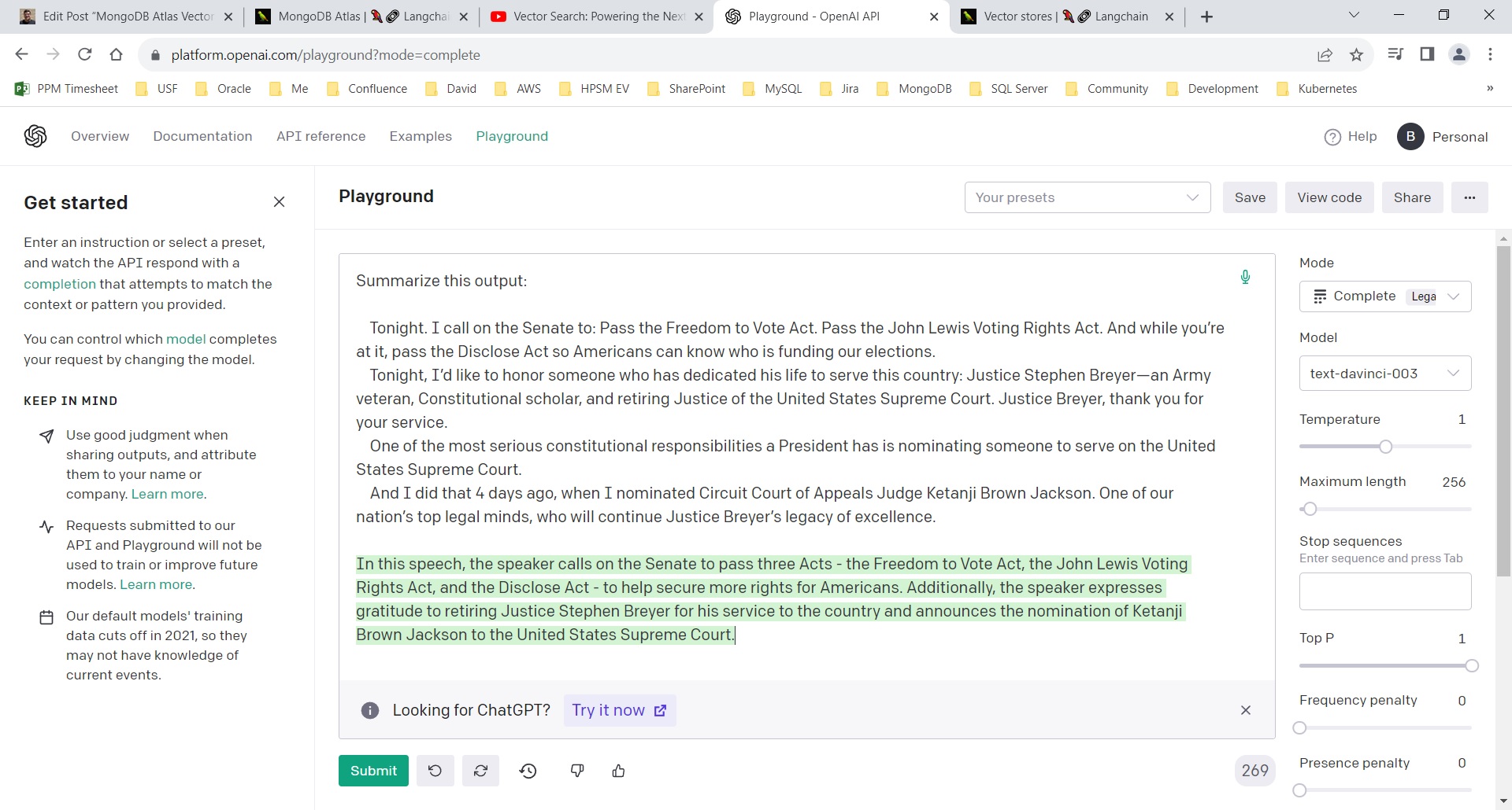
So, our programming project involved pulling in documents that were split up into pieces and then retrieve a piece based on a similarity query using the vector store and then ran that piece through OpenAI to generate a readable English summary.
Install MySQL 5.7.38 from source on Oracle Linux 8
This is a follow up to my earlier post about installing various MySQL versions from source:
https://www.bobbydurrettdba.com/2019/05/22/mysql-source-installs-for-each-rds-version/
So, I am an Oracle database administrator. I have been for about 30 years starting with Oracle 7. But for the past few years we have been supporting MySQL in Amazon Web Services’ RDS version. Unfortunately, we have been forced to embrace the Aurora version of MySQL also which is proprietary to Amazon and does not have the full source code. But we still have several vanilla MySQL RDS instances that we support.
Working with Oracle for so many years I have tried to learn about its internals – how does it really work? This is difficult because I do not have access to Oracle’s source code and even if I did, I probably do not have enough years remaining in my life to ever fully understand it. Still, the idea of working with the MySQL community edition version that we have the full source code to has always intrigued me. This is similar to my fascination with the antique computer game Nethack that I play in a character-based mode exploring a dungeon and fighting monsters. It is a good game, but more importantly, I have the full source code.
Who knows? Maybe when we are working with MySQL we will run across a bug, and I will be able to dig into the part of the code that has the bug and it will help me figure out how to solve the problem. With Oracle it is always a guess what is going on. It can be an educated guess based on what Oracle reveals through various traces and logs. But maybe even though I do not have the time and motivation to be a hardcore MySQL internals developer there could be a situation where having the source code will help.
So, that leads me to want to download the exact version of the MySQL source code that we are using on AWS RDS and compile it, link it, install it on a test VM on the chance that someday I will need a working test MySQL database of the same version as one that is having a problem in production.
Things have changed since my 5/22/2019 post about setting up this kind of environment. At that time, I was working with an Oracle Linux 7 VM running on my work laptop with all its firewalls and Zscaler and all between my VM and the internet. Today I am using Oracle Linux 8 running on a VM on a personal laptop which is on my home network so there is nothing in the way of my downloading things from the internet like Linux rpm packages. One of the side effects of COVID-19 is that I am working from home full time. Also, not due to COVID, my middle daughter moved out leaving her bedroom open to be converted to an office. So, I have two “desks” setup with two laptops and big monitors on both. My home laptop sits to my left and I can run VirtualBox VMs on it without being on our corporate network. This is great for testing where I just need to setup a technology and I do not need or even want access to something on our corporate network.
So, with all this prelude let me tell you some of the things I had to do to get the MySQL 5.7.38 source code compiled on my Oracle Linux 8 VM.
I cloned a OEL 8 VM that I already had and then updated the packages. I think I used yum instead of dnf which was dumb, but it worked.
Once I had an up-to-date OEL 8 environment I had to get the source tree for MySQL with the right commit point for 5.7.38. I was following this document:
https://dev.mysql.com/doc/refman/5.7/en/installing-development-tree.html
I ran these git commands:
git clone https://github.com/mysql/mysql-server.git

git checkout 5.7

git pull

This gets 5.7.38:

git checkout c94ce78
I installed Boost and Cmake like what I did in the earlier post. I got the rest of the development tools like gcc, make, bison in place using this dnf command:
dnf groupinstall "Development Tools"Then I had to get the cmake command to work:
cmake . -DWITH_BOOST=/home/bobby/boost_1_59_0I had to install several packages before I could get this to run without errors. I had to enable the “CodeReady Builder” repository in the file oracle-linux-ol8.repo:
[root@localhost yum.repos.d]# diff oracle-linux-ol8.repo oracle-linux-ol8.repo.06212023
20c20
< enabled=1
---
> enabled=0

[ol8_codeready_builder]
name=Oracle Linux 8 CodeReady Builder ($basearch) - Unsupported
baseurl=https://yum$ociregion.$ocidomain/repo/OracleLinux/OL8/codeready/builder/$basearch/
gpgkey=file:///etc/pki/rpm-gpg/RPM-GPG-KEY-oracle
gpgcheck=1
enabled=1
Once that repository was enabled, I was able to add the needed packages.
dnf install ncurses-devel
dnf install libtirpc-devel
dnf install rpcgen
Eventually I realized that after messing with adding the new repository and packages I needed to go back and clean everything up and run cmake again:
make clean
rm CMakeCache.txt
cmake . -DWITH_BOOST=/home/bobby/boost_1_59_0
make
su -
make install
Other than that, it is just the normal steps to create the database and run it, which I think is documented in my earlier post and in the MySQL docs.
I thought it couldn’t hurt to document the things I had to do if nothing else for myself. I use this blog as a reference for myself, so it is not just something for other people to read. Anyway, I’m glad I could get this down and maybe someone else will benefit.
Bobby
Full Database Restore and Recovery
Friday, we had to do a full restore and recovery of a production Oracle database. We used a script like this:
rman target / <<EOF

run {
allocate channel 'dev_0' type 'sbt_tape'
 parms 'SBT_LIBRARY=/opt/omni/lib/libob2oracle8_64bit.so,ENV=(OB2BARTYPE=Oracle8,OB2APPNAME=MYDB,OB2BARLIST=VTL_myhost_MYDB_oral1)';
allocate channel 'dev_1' type 'sbt_tape'
 parms 'SBT_LIBRARY=/opt/omni/lib/libob2oracle8_64bit.so,ENV=(OB2BARTYPE=Oracle8,OB2APPNAME=MYDB,OB2BARLIST=VTL_myhost_MYDB_oral1)';
allocate channel 'dev_2' type 'sbt_tape'
 parms 'SBT_LIBRARY=/opt/omni/lib/libob2oracle8_64bit.so,ENV=(OB2BARTYPE=Oracle8,OB2APPNAME=MYDB,OB2BARLIST=VTL_myhost_MYDB_oral1)';
allocate channel 'dev_3' type 'sbt_tape'
 parms 'SBT_LIBRARY=/opt/omni/lib/libob2oracle8_64bit.so,ENV=(OB2BARTYPE=Oracle8,OB2APPNAME=MYDB,OB2BARLIST=VTL_myhost_MYDB_oral1)';
allocate channel 'dev_4' type 'sbt_tape'
 parms 'SBT_LIBRARY=/opt/omni/lib/libob2oracle8_64bit.so,ENV=(OB2BARTYPE=Oracle8,OB2APPNAME=MYDB,OB2BARLIST=VTL_myhost_MYDB_oral1)';
allocate channel 'dev_5' type 'sbt_tape'
 parms 'SBT_LIBRARY=/opt/omni/lib/libob2oracle8_64bit.so,ENV=(OB2BARTYPE=Oracle8,OB2APPNAME=MYDB,OB2BARLIST=VTL_myhost_MYDB_oral1)';

restore database;
recover database
 delete archivelog maxsize 100 G;

}

exit
EOF
We ran it like this:
nohup ./restoredb.sh > restoredb.txt &The only tricky thing was getting the allocate channel commands right to work with our backup system (HP Data Protector). We had old examples of past recoveries, and we looked in Data Protector to see how the backup job was setup and what output the last backup produced.
Some storage work that we were doing accidentally damaged a bunch of data files. Fortunately, our control files and redo logs were intact, so we were able to fully recover and did not lose any data.
Bobby
LOB Space Scripts
I said in my previous post that I put LOB space scripts in my GitHub repository and I wanted to explain a little more here. I have two databases that were growing rapidly and the top segment in each was a LOB segment. For one database the top LOB was a CLOB and for the other it was a BLOB. In both cases there were many inserts and deletes against the tables with the largest LOB segment. I was trying to find out if space was wasted and unusable in the LOB segments. Best I can tell these applications are reusing space when LOBs are deleted. These were both BasicFiles LOBs in 11.2 Oracle. And for the CLOB the character set was such that each character used one byte. Also, both databases had an 8192-byte block size.
A lot of this work was inspired by this Oracle support document:
LOB space not released after delete (Doc ID 2285007.1)
The title made me think the LOB space was wasted after the deletes. But this article had an interesting disclaimer highlighted in a box:
“Note: be aware that the unused space after deletion can be reused in the
LOB segment for further insert after retention time is passed.”
As far as I can tell, Oracle’s disclaimer is correct, at least in our situation. Unused LOB space left after a deletion is reused.
Here is a description of the LOB scripts in my GitHub repository:
spacetest.sql – This was my first script. I used various versions of this script to test different metrics that I could find about LOBs. This was helpful because I started very simple and tried to understand what each source of information was telling me. I really struggled to understand what AVG_ROW_LEN from USER_TABLES was telling me until I realized that I was hitting this bug or one like it:
Bug 14651892 AVG_ROW_LEN computed incorrectly on LOB when AUTO_SAMPLE_SIZE is used
It also took me a long time to understand why DBMS_SPACE.SPACE_USAGE only reported full or unformatted blocks for LOB segments. LOBs are all or nothing for a block. Each LOB that is not stored inline for a row fully occupies one or more blocks. With all these observations I throw in the caveat that this is the best I can tell based on my observations on my system.
The database with the CLOB uses this character set: WE8MSWIN1252.
This Oracle document says that character sets like this have a single byte per character in a CLOB:
CLOBs and NCLOBs character set storage in Oracle Release 8i, 9i, 10g and higher (Doc ID 257772.1)
“CLOBs when using fixed width character set NLS_CHARACTERSET are stored in the NLS_CHARACTERSET character set on disk. Examples are WE8MSWIN1252 …”
This matters because dbms_lob.getlength returns the size of a CLOB in characters. In some character sets like AL32UTF8 you have to multiply dbms_lob.getlength’s output by 2 to get the bytes for the CLOB.
Given all the information I got from playing with spacetest.sql I created the next two scripts to feed information into the final space script.
blobinlinecutoff.sql – Takes an integer from 1 to 8191 and creates a row in a table with a LOB of that many bytes in size and it outputs whether that LOB is an inline LOB or not. I used this to find the cutoff point between LOBs that fit in a row and ones that did not. I found the cutoff to be 3964 bytes in all the scenarios I tried. I use this cutoff to ignore inline LOBs when counting the total LOB space in the column’s LOB segment.
inoneblock.sql – Takes an integer from 1 to 8191 and creates a row in a table with a LOB of that many bytes in size and it outputs whether that LOB fits fully in one block. Many LOBs are larger than one block which is only 8K for me so I wanted to calculate exactly how many blocks each LOB would take. I got 8132 in my tests which means 60 bytes per block are unusable for LOB storage. So, I would need to divide the LOB size in bytes by 8132 and round the resulting number up to the next integer to get the number of blocks occupied by the LOB.
I plugged the results from blobinlinecutoff.sql and inoneblock.sql into my final script:
lobspace.sql – Outputs information about LOB space used to show how much is allocated but not used by current LOBs. This space could either be available for reuse by future inserts or it could be wasted due to some bug.
Notice that the top of the script has the input from the previous two:
  inlinecutoff number := 3964;
  usableperblock number := 8132;
You also put the table owner, name, and LOB column name at the top as parameters.
The output looks like this on my BLOB column table:
--------------------------------------
Table owner = MYOWNER
Table name = MYTABLE
LOB column name = MYLOBCOLUMN
--------------------------------------
Number of rows in table = 380553608
Number of rows with lob in table row = 338491004
Number of rows with lob in lob segment = 42062604
Total lob segment size = 1496535 megabytes
Total size of full lob segment blocks = 1473933.135288238525390625 megabytes
Total lob space used in lob segment = 1462133.555019378662109375 megabytes
--------------------------------------
Percentage of full blocks used = 99%

PL/SQL procedure successfully completed.

Elapsed: 07:46:50.26
I found that this database is not deleting all the rows that it is supposed to, so it is fully using all the space freed by the deletes and is continually adding space.
But the output from the other database (the one with the CLOB) looked different:
--------------------------------------
Table owner = MYOWNER2
Table name = MYTABLE2
LOB column name = MYLOBCOLUMN2
--------------------------------------
Number of rows in table = 66360290
Number of rows with lob in table row = 54200592
Number of rows with lob in lob segment = 12159698
Total lob segment size = 913999 megabytes
Total size of full lob segment blocks = 906413.57425689697265625 megabytes
Total lob space used in lob segment = 373804.97021484375 megabytes
--------------------------------------
Percentage of full blocks used = 41%

PL/SQL procedure successfully completed.

Elapsed: 00:45:22.57
Notice that the percentage of full blocks used in the first database was 99% but in this one it is 41%. This made me really wonder if deleted space was really being freed for use by inserts. But digging further I found that we only keep 7 days of history on this table and back in November we hit a peak of activity which expanded the LOB segment. Since then, we have stopped adding new space to the LOB segment’s tablespace. It appears that we have plenty of space free for this LOB segment to absorb a new batch of inserts because more than half of the space in the LOB segment is free for reuse.
Here are the settings for the BLOB:
LOB (MYLOBCOLUMN) STORE AS BASICFILE (
  TABLESPACE  MYTABLESPACE
  ENABLE      STORAGE IN ROW
  CHUNK       8192
  RETENTION
  CACHE
  LOGGING
Here are the settings for the CLOB:
LOB (MYLOBCOLUMN2) STORE AS BASICFILE (
  TABLESPACE  MYTABLESPACE2
  ENABLE      STORAGE IN ROW
  CHUNK       8192
  RETENTION
  NOCACHE
  LOGGING
Some blog posts that I studied for this:
https://asktom.oracle.com/pls/apex/asktom.search?tag=reclaimreuse-lob-space
https://jonathanlewis.wordpress.com/2017/01/26/basicfile-lobs/
https://jonathanlewis.wordpress.com/2022/07/20/lob-space-2/
I wanted to put this out there to help others but also myself. I do not want to forget some of the things I learned in the process. Also, if anyone out there has any feedback on this including any errors that I made it would be great to hear it.
Bobby
LOB Scripts in my GitHub Repository
I do not have time to write a post explaining these now, but I wanted to note that I am posting LOB space related scripts here:
https://github.com/bobbydurrett/OracleDatabaseTuningSQL/tree/master/lob
Bobby
December 26 Plan Change
On December 26th, which is a holiday for my company this year, our team got a page that a plan had changed on an important 11.2.0.3 HP Unix platform Oracle database. The new plan was inefficient but did not cause any harm to the application. I added the SQL_ID value for the query to our plan change monitor exception list so that it would not page us again when it changes to slower plans because the slower plans were not a threat to the system. Normally I would just move on but this time I thought I would dig into why the query changed plan and see if there is anything we could do to prevent similar changes. If the new plan was a problem, I typically would force the faster plan with a SQL Profile. I was going to do that this morning, but the system was busy, and the profile script was hung up for a few minutes on a library cache lock, so I just backed it out. I do not really need to intervene since it is not hurting the system. We have enough CPU capacity to handle the slow plan. But I was still curious if I could find the underlying cause of the plan change and learn any lessons from it. That is what this post is about.
Like many queries that change plan and set off alerts, this problem query uses bind variables. The PL/SQL package that includes the queries passes in values in the where clause instead of using constants. I.e., it looks like this:
WHERE
    div = p_div
    AND cust_nbr = p_cust_nbr
and not this:
WHERE
    div = 123
    AND cust_nbr = 456
You can see here where the query changed to the bad plan:
PLAN_HASH_VALUE END_INTERVAL_TIME     EXECUTIONS_DELTA Elapsed Average ms
--------------- --------------------- ---------------- ------------------
      504369030 25-DEC-22 04.00.45 AM              838         .478386635
      504369030 25-DEC-22 07.00.40 PM             1599         .669989368
      504369030 25-DEC-22 11.00.15 PM             1044         .595122605
      504369030 26-DEC-22 01.00.16 AM              891         .558159371
      504369030 26-DEC-22 02.00.43 AM              473         .453122622
     2693825138 26-DEC-22 02.00.43 AM              311         3.61250804
     2693825138 26-DEC-22 03.00.07 AM              779         2.91877792
     2693825138 26-DEC-22 04.00.10 AM             1076           7.274671
     2693825138 26-DEC-22 05.00.41 AM             1218         11.1912258
The bad plan is averaging 11 milliseconds instead of less than 1 millisecond so “bad” is relative. It still is not slow enough to affect the users.
I used my plan script to run the problem query with different constants in place of the two variables. I used my optimizer statistics scripts to find what the optimizer thought the range of possible values was for the two columns. Here are the ranges:
COLUMN_NAME LO   HI
----------- ---- --------
DIV         228  5220
CUST_NBR    1675 74394502
I tried a variety of variable value combinations in and out of this range and most of the values outside these ranges resulted in the bad plan having a lower cost than the good one. It was especially sensitive to the values of DIV. It turns out that there are many possible DIV values outside this range. They are just not on this table. So likely this query is often run with variable values that are out of the range of what the optimizer knows is in the table.
I tried to find a way to make the out-of-range values pick the better plan. I loaded this data on a 19c database but got the same results. I tried different kinds of histograms, including one on (DIV, CUST_NBR), but they didn’t help.
So what?
Maybe when you write a query that takes variables you should try out its performance with atypical values for the variable values. In simple equals conditions like those in my problem query maybe check how the query runs on values that are outside of those found in the table. Since the query’s plan is not fixed you must be prepared for the query to run with all the plans that the data passed into its variables could generate. Also, the database will stick with any of those plans for a long time unless something forces it to be recalculated. So, you would have to test the query with atypical values and once the plan is in memory run all your typical data through that plan to see if it is still fast enough. If the plan from the atypical data is too slow then you would have to change the query or the data to handle those cases or resort to something like a hint to lock in the plan that runs well with the more typical variable values.
Bobby
P.S.
I just want to say how hard it is to write a blog post. What a pain. But the interaction with others on the internet is very valuable.
Someone commented that I could look at v$sql_shared_cursor to find why 1anm65yacs6ky changed plan. As expected, it changed plan because statistics were gathered on the table. Often statistics gathering causes plans to be recreated (hard parsing). But it was interesting that the reason from v$sql_shared_cursor was “Rolling Invalidate Window Exceeded”. A quick Google search led me to this article:
https://www.dbi-services.com/blog/oracle-rolling-invalidate-window-exceeded3/
It claims that there is a 5 hour window after statistics are gathered for plans to be reparsed. This makes sense because I know statistics are gathered on the table around 22:00 but the plan is flipping between 01:00 and 02:00 the next day. Very cool.
But it does not really explain why the plan changes. It only explains why 1anm65yacs6ky was hard parsed. The plan changed because out of range data was passed into the bind variables during the hard parse and this resulted in a plan that was inefficient for in range data. On December 26th we got unlucky during the hard parse. This morning, January 9th, we got lucky, and we flipped back to the good plan.
What makes blogging about this stuff so hard is that there is so much I want to say about this, but I just don’t know if I have the energy or ability to put it all down. We use bind variables to minimize parsing. With the good plan this query runs in a couple of milliseconds. If it had to be hard parsed every time it runs, 14,000 times per hour, it would be very wasteful and slow. But the cost of using bind variables is that a plan can get locked in that isn’t efficient for many of the values passed into the variables. It is a no-win scenario. The bigger picture is that I think Oracle’s optimizer, and probably any conceivable SQL optimizer, has limits. Somehow all these years Oracle and others have produced SQL RDBMSs that people find useful. But based on my Oracle experience it seems like they are imperfect but useful.
In the case of my December 26th query that changed plan, our business is functioning just fine with the query’s plan flipping back and forth. If I did not have my plan change monitor setup, I would not even know that the plan was changing because it is not causing an issue that is visible to the users. So, it offends my perfectionist tendencies to have a query run an inefficient plan, but from a business perspective the inefficiency and imperfection that is fundamental to the design of Oracle’s optimizer with the tradeoffs of minimizing hard parses with bind variables but suffering with inefficient plans until the next hard parse is acceptable because the business purpose of the application is still being accomplished. Maybe in the bigger picture Oracle’s SQL and SQL in general have been useful to people all these years because they do well enough to meet people’s needs despite their fundamentally imperfect execution of SQL queries.
P.P.S.
I found two ways to prevent the SQL statement from changing plans when it is hard parsed with variable values that are out of the range of the column statistics. One is to add a new index, and the other is to add a cardinality hint.
I had no idea if the index would help but I noticed that the query touched the same table 3 times after looking up rows using the only index. I looked at the subselects on the query and picked a new index that would cover all the columns used by the subselects and be efficient. This eliminated all but the one table lookup that we had to have. For some reason this plan is chosen even if the data in the variables is out of range. Maybe the new index made the plan so efficient that out-of-range data would not cause a plan flip.
Just now I got the idea of trying a cardinality hint like this:
/*+ cardinality(PSD 10) */I put this on every subselect that had the main table. This caused the plan to act as if the table would return 10 rows and it choose the good plan even if the data in the variables was out of range.
These two approaches work but they require some query tuning knowledge when you are rolling out new SQL statements. I think part of the challenge of using SQL databases like Oracle is that you need developers and DBAs who understand the optimizer well enough to understand the challenges of bind variables and plan changes and how to prevent them or fix them.
P.P.P.S.
See this Oracle support document:
Limitations of the Oracle Cost Based Optimizer (Doc ID 212809.1)
There is also this bug which may prevent us from using Adaptive Cursor Sharing on this application which has all its queries wrapped in PL/SQL:
Bug 8357294 : ADAPTIVE CURSOR SHARING DOESN’T WORK FOR STATIC SQL CURSORS FROM PL/SQL
It looks like none of our SQL is using ACS:
>select
  2  IS_BIND_SENSITIVE,
  3  IS_BIND_AWARE,
  4  count(*) cnt
  5  from
  6  v$sql
  7  group by
  8  IS_BIND_SENSITIVE,
  9  IS_BIND_AWARE
 10  order by cnt desc;

I I        CNT
- - ----------
N N      22970
Maybe our application design suppresses the use of ACS which results in more bad plans being locked in on queries with bind variables. If we bypassed PL/SQL and just ran queries against the database from the Java front end, we might use ACS to prevent a bad plan getting locked in based on certain oddball variable values.
1/12/22
Tired of writing PPS and all that. I am probably running out of steam. I cannot find anything that really applies generally to our system based on this example. I found this weird part of the plan when the variable values are out of range:
------------------------------------------------------------------------
| Id  | Operation                            | Name            | Rows  |
------------------------------------------------------------------------
|   6 |       MERGE JOIN CARTESIAN           |                 |     1 |
|   7 |        TABLE ACCESS BY INDEX ROWID   | PROD_ATLN_DTL   |     1 |
|   8 |         INDEX RANGE SCAN             | PROD_ATLN_DTL_0 |     1 |
|   9 |        BUFFER SORT                   |                 |    36 |
|  10 |         TABLE ACCESS FULL            | XYZ_ENT         |    36 |
It seems like for Id 6 the Rows value should be 36 instead of 1. I think the optimizer treats 0 rows as 1 row when it displays the plan so maybe it is multiplying 0 * 36 and then displaying 1 instead of 0 for id 6. But other parts of the plan treat 0 as if it was 1 and add up the cost of the steps of the plan. Both the good and bad plan have costs that are way off for the out of range variable values so maybe when you get down to this level the errors inherent in the optimizer make plan comparisons meaningless. But then what strategy can you use with queries that use bind variables and that have out-of-range data values passed into them? You can use hints, etc. but what can you do without intervening for every query like this?
1/13/22
Looks like the cartesian joins were caused by the constants being in the query in two places.
In the innermost subselect it was this:
   WHERE     DIV = 111
         AND CUST_NBR = 222
Then in the final where clause:
 WHERE     PCD.DIV = 111
       AND PCD.CUST_NBR = 222
DIV and CUST_NBR where part of the joins all through the query so these constants were only needed once. Ultimately this query was poorly constructed, so the optimizer had trouble locking down a good plan. Maybe the bigger picture is that the better job we do designing our queries, indexes, etc. the less likely plans are to change for the worse.
US Foods IT Hiring
Gold image for 19.16 install on RHEL 8
On Red Hat 7 Linux VMs we use a zip of a 19c Oracle home with the latest quarterly database release update applied which at the moment in 19.16, the July 19, 2022 version. Our standard deployment script just unzips the gold image zip and then runs the installer silently with a response file. But when I ran the same process on a Red Hat 8 VM I got errors. I found something that said to set this variable to resolve the first error:
export CV_ASSUME_DISTID=’OL7′
And then I got package missing errors which I could ignore about this package:
compat-libcap1-1.10.
But I finally hit an error that I could not get around no matter what I did:
[FATAL] Error in invoking target ‘all_no_orcl’ of makefile ‘/oracle/product/db/19.0.0.0/rdbms/lib/ins_rdbms.mk’.
So, I opened a service request (SR) with Oracle support, and they gave me a series of steps to rebuild my 19.16 gold image zip in a way that would get past this error. There was only once step that I had to add to what they recommended so I want to document that here.
First, they recommended unzipping the base 19.3 install file in my oracle home and then putting in the current opatch. These steps looked like this on my system:
unzip LINUX.X64_193000_db_home.zip -d $ORACLE_HOME
cp p6880880_190000_Linux-x86-64.zip $ORACLE_HOME
cd $ORACLE_HOME
mv OPatch OPatch.orig
unzip p6880880_190000_Linux-x86-64.zip
This just left me with the base 19.3 install and the current opatch in the Oracle home but nothing installed.
Through a bunch of trial and error I found that I needed this step before I went further:
cp /etc/oraInst.loc /oracle/product/oraInventory
Our VMs come with an OEM client pre-installed so there is already an inventory. Maybe that is why I needed this step. I have not had a chance to test this on a clean RHEL 8 VM without an OEM client installed.
Next, I had to run the actual install which required an X server with the DISPLAY variable setup. I had fun getting this to work with MobaXterm and its ssh tunnel feature but once I figured it out it worked great. I ended up setting my DISPLAY variable like this:
export DISPLAY=localhost:0.0
I set the tunnel to listen on port 6000 on my RHEL8 vm and connected it to that same port on the ip for my MobaXterm X server. Maybe that needs a separate post, but other people probably do this all the time.
The install uses this patch:
Patch 34160854: COMBO OF OJVM RU COMPONENT 19.16.0.0.220719 + GI RU 19.16.0.0.220719
I unzipped this to /oracle/db01/install/34160854
Then I ran the install like this:
./runInstaller -applyRU /oracle/db01/install/34160854/34130714
This spit out some text messages about applying the patch but then went into the normal graphical interactive installation steps through X windows. I did a standalone binary install without RAC.
Next, I had to apply the other part of the combo patch:
$ORACLE_HOME/OPatch/opatch apply /oracle/db01/install/34160854/34086870
This ran like a typical opatch apply.
Now that I had followed Oracle’s instructions to install 19.16 in a way that could be made into a gold image that works on RHEL 8 I did the following to make the gold image:
./runInstaller -silent -createGoldImage -destinationLocation /oracle/db01/install
Then I blew away everything in the oracle home and the inventory directory and redid the install from the new gold image like this:
unzip /oracle/db01/install/db_home_2022-09-20_05-53-23PM.zip -d $ORACLE_HOME
$ORACLE_HOME/runInstaller -silent -responseFile $ORACLE_HOME/19cresponsefile.rsp
The response file was the same that we always use for 19c on RHEL 7. Also, I did not need to set CV_ASSUME_DISTID=’OL7′ because the gold image has a recent version of the installer that does not require it. I think the main point of installing from patch 34160854 was to get a patched version of the installer that works with RHEL 8. My old gold image zip was made from the base 19.3 zip with the 19.16 database release update applied. Evidently that did not update the installer to make it support Red Hat 8, so I had to build a new gold image using patch 34160854 as described above.
Anyway, I don’t have a ton of time to go back and clean all this up right now but hopefully this basic dump of information will be helpful to someone. If nothing else, it will remind me!
Bobby