


Yann Neuhaus


Fixing ORA-00904 on Oracle hidden columns during SSMA data migration
SSMA (SQL Server Migration Assistant) handles the whole Oracle-to-SQL Server move: it reads the source data dictionary, converts the schema, then generates a SELECT per table to pull the rows across. That last step is where this story goes wrong.
The problemMigrating ~5,600 Oracle tables to SQL Server with SSMA. Most load fine; ~100 tables fail Migrate Data with the same error:
ERROR [42S22] [Oracle][ODBC][Ora]ORA-00904:
"SYS_C00004_21081414:28:22$": invalid identifier
The named column exists in no DDL anyone wrote. The [Ora] prefix says Oracle itself is rejecting the query: SSMA built an extraction SELECT naming a column Oracle refuses to resolve. Tellingly, SELECT * and COUNT(*) run fine against the same table, whatever this column is, Oracle is happy to ignore it, but not to be asked for it by name.
The name is the giveaway: SYS_C00004_21081414:28:22$ is what Oracle calls a column after ALTER TABLE … SET UNUSED COLUMN.
Oracle offers two ways to get rid of a column: a logical delete and a physical one. The physical delete (ALTER TABLE … DROP COLUMN) is the honest one, but on a large table it is very time- and resource-consuming. That’s why people reach for the logical delete instead:
ALTER TABLE table_name SET UNUSED (column_name);
That statement is metadata-only and instant. The column immediately stops being visible to users, and the physical removal is deferred to whenever there is time for it (see Oracle Documentation):
ALTER TABLE table_name DROP UNUSED COLUMNS;
-- on large tables, cap undo growth by checkpointing every N rows:
ALTER TABLE table_name DROP UNUSED COLUMNS CHECKPOINT 250;
To free the original name for reuse, Oracle renames the column to SYS_C<internal column number>_<YYMMDDHH24:MI:SS>$, sets USER_GENERATED to NO, HIDDEN_COLUMN to YES and releases its COLUMN_ID. So the timestamp is not when the column was added, it is the second someone ran SET UNUSED. Ours says 14 August 2021, 14:28:22.
That also explains the error pattern. The operation is one-way and the column is unreadable by design, so naming it gets you ORA-00904 «invalid identifier». SELECT * and COUNT(*) keep working because the column no longer has a COLUMN_ID and is simply excluded from the star. SSMA, however, lists it and builds an explicit column list Oracle then refuses.
Not to be confused with SYS_NC…$. Those are a different animal: virtual columns backing a function-based index or extended statistics.
Bottom line: returning NULL costs you nothing. This is a column its owner already decided to delete, holding data Oracle itself will no longer hand out. There is no information left to lose.
What doesn’t work for the migration- SSMA setting
Ignore hidden system columns = Yeswas not making any effect on this use case - Dropping the column on SQL Server resolves nothing because the error is on the source SELECT, unaffected.
- Dropping it on Oracle could not be done in our scenario because the source is frozen; DDL not allowed.
- Custom select, column removed or bare
NULL: SSMA still expects the name in its mapping and fails with “key not present” or “does not match up” before the query ever reaches Oracle.
Before editing anything, get the full list. Discovering the affected tables one failed migration at a time is a waste of an afternoon because the data dictionary already knows.
The reason the columns are findable at all is an asymmetry between two views: an unused column is gone from ALL_TAB_COLUMNS, but still listed in ALL_TAB_COLS with HIDDEN_COLUMN = 'YES'. That second view is what you query:
SELECT owner,
table_name,
column_name,
data_type,
internal_column_id,
TO_DATE(REGEXP_SUBSTR(column_name, '\d{8}:\d{2}:\d{2}'),
'YYMMDDHH24:MI:SS') AS set_unused_at
FROM dba_tab_cols
WHERE hidden_column = 'YES'
AND user_generated = 'NO'
AND REGEXP_LIKE(column_name, '^SYS_C\d+_\d{8}:\d{2}:\d{2}\$$')
-- AND owner = '<SCHEMA_NAME>'
ORDER BY owner, table_name, internal_column_id;
The regex is deliberately strict: it matches only the SET UNUSED naming pattern, so virtual columns and other system-generated names stay out of the result.
One more view is worth a look, as a cross-check:
SELECT owner, table_name, count AS unused_columns
FROM   dba_unused_col_tabs
--WHERE owner = '<SCHEMA_NAME>'
ORDER  BY count DESC, table_name;
DBA_UNUSED_COL_TABS gives the number of unused columns per table. Sorting by that number puts the dangerous tables first: those with two or three hidden columns are the ones where you’ll forget a line in the custom select and be back at square one.
Keep the hidden column’s name as an alias, but return a literal NULL instead of reading it. SSMA’s mapping finds the name (no “key not present”); Oracle never resolves the real column (no ORA-00904).
- Tools → Project Settings → General → Migration → enable Extended data migration options.
- Data Migration Settings tab → tick Use custom select → replace each hidden-column line with:
 SELECT ...
    TO_CHAR("<COLUMN_NAME>", 'TM', 'NLS_NUMERIC_CHARACTERS = ''.,''') as "<COLUMN_NAME>",
    NULL as "SYS_C00004_21081414:28:22$"
from <OWNER>.<TABLE_NAME> t
- Migrate Data → 100%. Drop the NULL-filled column(s) on SQL Server in post-migration cleanup.
SYS_C…$ is not an exotic Oracle feature, it’s an ordinary column someone deleted years ago, logically. Oracle keeps the name on file; SSMA finds it, insists on naming it, and Oracle refuses to hand it over. Aliasing a NULL satisfies both, then you drop the column on the target. No source DDL, no external tooling, everything inside SSMA, behind a project setting that’s hidden by default.
L’article Fixing ORA-00904 on Oracle hidden columns during SSMA data migration est apparu en premier sur dbi Blog.
NGINX Secured Distribution Path with GoldenGate REST API
In a previous blog, I presented how to set up a distribution path between two GoldenGate deployments both secured with NGINX. The method I used there was purely through the Web UI. But GoldenGate also exposes a full REST API, and everything you can do in the UI can be done through the API as well, which is useful for automation, scripting, or when the UI is not reachable.
This blog covers the exact same setup, using the REST API instead. I will show two ways of doing it :
- Using
oggrestapi.py, the GoldenGate REST client I released in another blog. - Using the
requestslibrary to call the REST API directly.
The prerequisites are the same as in the previous blog :
- Two GoldenGate Microservices deployments,
ogg_test_01(source) onoggvm1andogg_test_02(target) onoggvm2. I will use the latest 26ai version. - Both OGG setups secured with NGINX acting as a reverse proxy, so everything goes through port
443. - A running extract on the source, writing to a trail (
aain my case).
Just like in the Web UI, there are three steps to get a working distribution path :
- Create a path connection on the source, to authenticate against the target.
- Register the target’s CA certificate on the source Service Manager.
- Create and start the distribution path.
A quick note on URLs before we start. Behind an NGINX reverse proxy, each service has its own path prefix :
- Administration Service :
/services/<deployment>/adminsrvr/v2/... - Distribution Service :
/services/<deployment>/distsrvr/v2/... - Service Manager :
/services/ServiceManager/v2/...
The oggrestapi.py client builds these for you as soon as you pass reverse_proxy=True and the deployment name, so let’s connect once and reuse the client. If you don’t provide the password argument, you will be prompted for it.
from oggrestapi import OGGRestAPI

ogg_source = OGGRestAPI(
    url="https://oggvm1",
    username="ogg",
    deployment="ogg_test_01",
    reverse_proxy=True,
)As explained in Creating Path Connections with GoldenGate REST API, a path connection is simply an alias in the Network domain. It stores the credentials of a user that exists on the target deployment, and its alias is only known on the source side.
With the client, just call the create_alias method :
ogg_source.create_alias(
    alias="ogg_target",
    domain="Network",
    data={
        "userid": "ogg_user_on_target",
        "password": "***",
    },
)
As mentioned in the introduction, here is the same call with requests, calling the Administration Service of oggvm1 through NGINX :
import requests

auth = ("ogg", "ogg_password")

response = requests.post(
    "https://oggvm1/services/ogg_test_01/adminsrvr/v2/credentials/Network/ogg_target",
    auth=auth,
    json={
        "userid": "ogg_user_on_target",
        "password": "***",
    },
)
After refreshing the source Web UI, the new path connection is visible under the Path Connections tab :

But of course, you can also view the new path connection by calling the REST API:
# Since path connections are aliases of the Network domain, we use the get_alias method to retrieve them
>>> ogg_source.get_alias('Network', 'ogg_target')
{'$schema': 'ogg:credentials', 'userid': 'ogg_user_on_target', 'type': 'PASSWORD'}Because the deployments are secured with NGINX, the source has to trust the certificate authority that signed the target’s certificate. This is done on the source Service Manager, by registering the target’s root CA certificate.
With the client, use create_deployment_certificate against the source deployment. The certificate type to use is truststore, and the certificate content goes under trustpointBundle.trustpointPem:
target_ca = open("rootCA_ogg_test_02.pem").read()

ogg_source.create_deployment_certificate(
    deployment="ogg_test_01",
    type="truststore",
    certificate="rootCA_ogg_test_02",
    data={
        "trustpointBundle": {
            "trustpointPem": target_ca,
        }
    },
)
The same call with requests, this time on the Service Manager prefix :
target_ca = open("rootCA_ogg_test_02.pem").read()

response = requests.post(
    "https://oggvm1/services/ServiceManager/v2/deployments/ogg_test_01/certificates/truststore/rootCA_ogg_test_02",
    auth=auth,
    json={
        "trustpointBundle": {
            "trustpointPem": target_ca,
        }
    },
)
Registering under the specific deployment (ogg_test_01) is the equivalent of the Local option in the Web UI. To get the Shared behavior instead, register the same certificate under the ServiceManager deployment name, so it becomes available to every deployment on that node.
If the certificate file contains a chain of certificates, you must register each certificate individually, since GoldenGate does not accept them in one go. I described that issue in detail in a blog about the OGG-30007 error.
We can now create the distribution path itself. It has a source endpoint (the local trail) and a target endpoint (the target’s Receiver Service, reached over wss through NGINX). Because the target is NGINX-secured, the target URI :
- uses the
wssprotocol on port443, - points at the Receiver Service path prefix,
recvsrvr, notdistsrvr(that prefix is only for the Distribution Service on the source side), - does not carry the path connection alias itself. The alias goes in a separate
authenticationMethodkey.
With the client :
ogg_source.create_distribution_path(
    distpath="path12",
    name="path12",
    source={
        "uri": "trail://localhost/services/v2/sources?trail=PDB1/aa",
    },
    target={
        "uri": "wss://oggvm2/services/ogg_test_02/recvsrvr/v2/targets?trail=PDB1/bb",
        "authenticationMethod": {
            "domain": "Network",
            "alias": "ogg_target",
        },
    },
    begin="now",
    status="running",
)
And the equivalent requests call, on the Distribution Service prefix (/services/ogg_test_01/distsrvr/):
response = requests.post(
    "https://oggvm1/services/ogg_test_01/distsrvr/v2/sources/path12",
    auth=auth,
    json={
        "name": "path12",
        "source": {
            "uri": "trail://localhost/services/v2/sources?trail=PDB1/aa",
        },
        "target": {
            "uri": "wss://oggvm2/services/ogg_test_02/recvsrvr/v2/targets?trail=PDB1/bb",
            "authenticationMethod": {
                "domain": "Network",
                "alias": "ogg_target",
            },
        },
        "begin": "now",
        "status": "running",
    },
)
The trail value in both URIs also has to match the path the extract actually registers, EXTTRAIL PDB1/aa on the source becomes trail=PDB1/aa in the source URI, and the same logic applies to the target’s bb trail. A bare trail=aa without the PDB path segment matches neither what the extract writes nor what the target’s own directory layout expects.
Once the path is created with status: "running", the trail files start flowing. You can confirm it on the target :
oracle@oggvm2:~/ ll $OGG_DEPLOYMENT_HOME/var/lib/data/PDB1
total 0
-rw-r-----. 1 oracle oinstall 0 Mar 22 07:34 bb000000000If your distribution path doesn’t start and generates a “certificate that failed validation” error, it means that you incorrectly registered your certificates. Make sure that the target deployment’s CA certificate is registered on the source Service Manager, and not the other way around.
And that’s it. With three REST calls, through oggrestapi.py or using the requests module, you get the exact same NGINX-secured distribution path as the Web UI method, but in a form you can script and repeat.
L’article NGINX Secured Distribution Path with GoldenGate REST API est apparu en premier sur dbi Blog.
GoldenGate 26ai out-of-place patching with Python
I already covered out-of-place patching from the web UI, but patching tasks should be automated, and clicking through the same screens for every deployment can get repetitive. Let’s do the exact same out-of-place patch of a GoldenGate Microservices Architecture deployment, this time entirely with the REST API.
Every step below shows two ways to make the same call:
- A standard
requestscall, the default Python module to handle REST APIs. - The equivalent call using
oggrestapi.py, theOGGRestAPIPython client I presented in another blog, which handles everything for you.
This part does not change: the REST API cannot install software on the server, so you still need to unzip the patched installation to a new OGG_HOME and run runInstaller in silent mode, as described in the web UI blog.
As with the web UI, the Service Manager has to be patched first. Assume the following setup:
sm_url:https://vmogg:7809new_ogg_home:/u01/app/ogg/product/23.26.2.0.1username/password: an administrator on the Service Manager
Updating OGG_HOME is a PATCH call on the ServiceManager deployment:
import requests

sm_url = "https://vmogg:7809"
auth = ("oggadmin", "password")

requests.patch(
    f"{sm_url}/services/v2/deployments/ServiceManager",
    json={"oggHome": "/u01/app/ogg/product/23.26.2.0.1"},
    auth=auth,
)
With oggrestapi.py:
from oggrestapi import OGGRestAPI

client = OGGRestAPI(url="https://vmogg:7809", username="oggadmin", password="password")
client.update_deployment(deployment="ServiceManager", ogg_home="/u01/app/ogg/product/23.26.2.0.1")
Already, you can see that the REST API client simplifies the patching a lot.
Restarting the Service Manager is the same endpoint, this time setting status:
requests.patch(
    f"{sm_url}/services/v2/deployments/ServiceManager",
    json={"status": "restart"},
    auth=auth,
)client.restart_deployment(deployment="ServiceManager")restart_deployment is a dedicated method in oggrestapi.py, following the same pattern already used for restart_service, restart_extract and restart_replicat. It makes it easier to use the API, instead of building the {"status": "restart"} payload yourself. It also takes an optional only_if_running argument, so a deployment that was already stopped before the patch is left alone rather than being started by the restart call.
As with the web UI, all your deployment processes are still running on the old OGG_HOME at this point. The AIService, introduced in 26ai, does not pick up the new home automatically either. You should then list the services attached to the Service Manager and restart the ones that are not ServiceManager itself:
services = requests.get(
    f"{sm_url}/services/v2/deployments/ServiceManager/services",
    auth=auth,
).json()["response"]["items"]

for service in services:
    if service["name"] != "ServiceManager":
        requests.patch(
            f"{sm_url}/services/v2/deployments/ServiceManager/services/{service['name']}",
            json={"status": "restart"},
            auth=auth,
        )
for service in client.list_services("ServiceManager"):
if service.get("name") != "ServiceManager":
client.restart_service(deployment="ServiceManager", service=service.get("name"))Once the Service Manager runs on the new home, repeat the same update, then restart sequence for each deployment (oggHome, then status: restart):
deployment = "ogg_test_01"

requests.patch(
    f"{sm_url}/services/v2/deployments/{deployment}",
    json={"oggHome": "/u01/app/ogg/product/23.26.2.0.1"},
    auth=auth,
)

requests.patch(
    f"{sm_url}/services/v2/deployments/{deployment}",
    json={"status": "restart"},
    auth=auth,
)
client.update_deployment(deployment="ogg_test_01", ogg_home="/u01/app/ogg/product/23.26.2.0.1")
client.restart_deployment(deployment="ogg_test_01")Once the deployment is back up, restart its extracts and replicats. Since these processes are not accessible through the Service Manager port, you need to change the URL. If you use a reverse proxy setup, or auto_discovery=True (see below), this is also easier with the Python client.
admin_url = "https://vmogg:7810"

extracts = requests.get(f"{admin_url}/services/v2/extracts", auth=auth).json()["response"]["items"]
for extract in extracts:
    requests.patch(f"{admin_url}/services/v2/extracts/{extract['name']}", json={"status": "stopped"}, auth=auth)
    requests.patch(f"{admin_url}/services/v2/extracts/{extract['name']}", json={"status": "running"}, auth=auth)

replicats = requests.get(f"{admin_url}/services/v2/replicats", auth=auth).json()["response"]["items"]
for replicat in replicats:
    requests.patch(f"{admin_url}/services/v2/replicats/{replicat['name']}", json={"status": "stopped"}, auth=auth)
    requests.patch(f"{admin_url}/services/v2/replicats/{replicat['name']}", json={"status": "running"}, auth=auth)
With oggrestapi.py, restart_all_extracts and restart_all_replicats do the same thing on an OGGRestAPI client already pointed at the deployment (either connected directly to its Administration Service, or through an NGINX reverse proxy with deployment= set):
admin_client = OGGRestAPI(url="https://vmogg:7810", username="oggadmin", password="password")
admin_client.restart_all_extracts(only_if_running=True)
admin_client.restart_all_replicats(only_if_running=True)The steps listed above (update home, restart deployment, restart processes for every deployment) is exactly what patch_deployment (a single deployment) and patch_deployments (all of them) already do in oggrestapi.py, internally calling restart_deployment for the restart step. They also handle the ServiceManager special case (patch and restart the deployment and its services, but never restart extracts and replicats on it) and the wait_until_deployment_status polling in between:
client = OGGRestAPI(url="https://vmogg:7809", username="oggadmin", password="password", reverse_proxy=True)
client.patch_deployments(new_home="/u01/app/ogg/product/23.26.2.0.1", ask_credentials=False)
Both methods take restart_after_patch and restart_processes_after_patch (both default to True) if you need to skip either step, for example to patch every home first and restart everything in a separate maintenance window:
client.patch_deployments(
    new_home="/u01/app/ogg/product/23.26.2.0.1",
    restart_after_patch=False,
    restart_processes_after_patch=False,
    ask_credentials=False,
)
restart_processes_after_patch=True needs per-deployment routing: restarting extracts and replicats on ogg_test_01 is a different call than on ogg_test_02, and a plain connection to the Service Manager’s own port has no way to reach either one. oggrestapi.py gives you two ways to get that routing from a single client:
reverse_proxy=True, shown above, if you already run NGINX in front of your deployments.auto_discovery=True, with no reverse proxy at all. The client looks up each deployment’s real Administration/Distribution/Performance Metrics Service port through the Service Manager itself (the sameGET .../deployments/{deployment}/services/{service}call), the first time each one is actually needed, and reuses that lookup for the rest of the run:
client = OGGRestAPI(url="https://vmogg:7809", username="oggadmin", password="password", auto_discovery=True)
client.patch_deployments(new_home="/u01/app/ogg/product/23.26.2.0.1", ask_credentials=False)
Without either flag, patch with restart_processes_after_patch=False and restart each deployment’s processes yourself through a separate client pointed at that deployment’s own admin URL.
OGG_HOME
Same as with the web UI: a restart call on a deployment returns as soon as the Administration Service (adminsrvr) is back up. The Receiver Service (recvsrvr) or the Distribution Service (distsrvr) can take a bit longer to restart. If, after polling for a few minutes, a service is still reporting the old home, restart it individually with the same PATCH .../services/{service} call shown above for the AIService, or with the restart_service method.
If you change the name of your home at every release, remember to update OGG_HOME in every script and environment that references it, for example:
- DMK environment files.
systemdservice files, which might hardcode theOGG_HOMEvariable.
L’article GoldenGate 26ai out-of-place patching with Python est apparu en premier sur dbi Blog.
M-Files Compliance Kit 2026 is available
Recently, I decided to conduct an initial test involving a review in one of our test environments. The aim was twofold: to explore the new features and to verify the update process. You can read about my experience and the outcome in this blog post.
In week 29 of 2026, M-Files released a new version of its widely known and used M-Files Compliance Kit. This is especially useful if you are looking for advanced workflow capabilities or working in a regulated environment. The Compliance Kit is an essential tool.
This first version of the 2026 edition was followed by several smaller updates and fixes, culminating in version 2026 (26.9.16376.0).In this blog, I will highlight some of the improvements that I consider significant. The full release notes can be found on the M-Files official website.
This does not reflect the complete list, but it does include some of the most important parts.
Features- Object Creator commands and groups can use custom icons (including your own SVG or image-based icons).
- You can create and arrange custom task bar groups, control their placement and priority, and merge them with built-in groups.
- Commands can be shown outside their group in the context menu to match the classic client’s layout.
- Existing configurations continue to work with no changes required — classic client behavior is preserved, and legacy icons are reused automatically in newer clients where appropriate.
- CAD File Preview Support
CAD files with extensions .dwg, .dxf, .dwt, and .dgn can be previewed within the new Clients Preview tab, utilizing the active layout. The maximum supported file size is 50 MB. Previews are generated using a converted PDF format. Administrators have the capability to enable this conversion process for workflow state transitions or on-demand PDF conversion through the “Configuration>PDF Conversion (Indexing, File Preview, Workflows)>CAD Files>Enable On-Demand Conversion” setting, which is disabled by default.
- Activity feed now identifies AI-driven changes
When an object’s metadata is edited automatically based on an AI response, the activity feed now shows “M-Files AI” as the editor instead of a generic “M-Files” entry, making it clearer when a change was made by AI rather than a person. - Icons in view listing columns
The new M-Files client now shows a small icon next to value-list values in view listing columns — Workflow, Workflow state, Class, Object Type, and any custom value list item — so users can recognise the state, class, and type of each object at a glance without opening it. - Improved metadata card appearance
The metadata card now correctly displays custom colors for property group headers and descriptions. This ensures a more consistent and visually clear experience when viewing object details. - Drag-and-drop support for relationships and document collection management
Users can now drag and drop one or multiple objects onto another object in the listing to add documents to a document collection, establish relationships, append files to a multi-file document, or replace a file’s content. - Edit documents stored in M365 Storage using Web Co-Authoring
You can now open and co-author documents directly in the Office Web version using the new ‘Edit in Web’ option in the context menu. This makes it easier to collaborate online without needing the Office Desktop application. - UIXv2: show multiple dashboards in a popup window
You can now display up to three dashboards side by side in a pop-up window using the UI extensibility framework (UIXv2). This helps you compare information and work more efficiently without switching views.
As previously mentioned, a large number of improvements have been made and many defects have been fixed. Please refer to the official M-Files documentation for further details.
Installation and Update processI can confirm that the installation and update process was very straightforward and worked without any issues. As always, you can simply install the new Vault Framework application in the Vault. There is no need to uninstall the previous version.
After installation, navigate to the Compliance Kit configuration in the Vault. As in previous versions, an update button will be displayed. Pressing this button starts the update process, which went very well in my test. Afterwards, the Compliance Kit worked as expected, with all configurations and settings remaining intact.

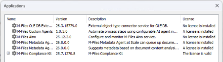
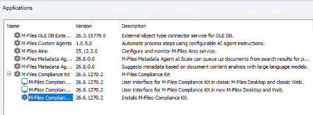
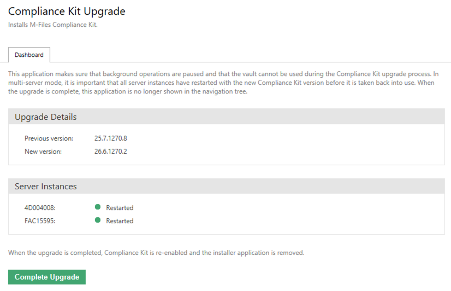
After restarting and refreshing the vault, the upgrade application is shown under configuration. Next, we can start the final update process by pressing the button, as shown in the screenshot.
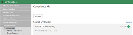
Once again, the M-Files Admin Tool is refreshed and the result of the update confirms that the new version of the Compliance Kit is 2026.
 Example of new features
The examples below demonstrates the new features of the M-Files Compliance Kit 2026, as implemented in a Quality Management System (QMS) demo vault.
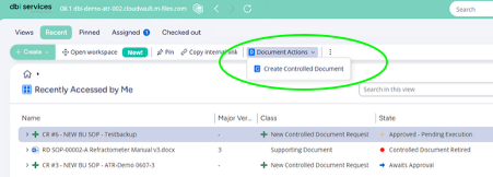
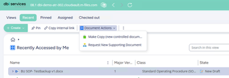
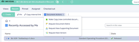
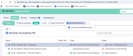
The picture below shows the new features based on an approved change request. Refer to the cycle in the picture to see the commands available for an approved change request. This makes it very easy to create a new document based on the approved change request.
This function was already available in the classic client but was sorely missed by almost every user in the new client.
 Web Client
 Conclusion
With all the improvements and fixes, particularly the new client’s command retrieval function. This is a step in the right direction. If you’re wondering how it works in the web client.Tthe answer is that anything that works in the new client also works in the web client.
If you have any questions or would like a demonstration, please get in touch with us. We can also assist with installation, updates and configuration.
L’article M-Files Compliance Kit 2026 is available est apparu en premier sur dbi Blog.
Information debt: The technical debt nobody talks about
When people hear the term “Technical debt”, they immediately understand what it means!
Take shortcuts today, pay the price tomorrow.
Everyone knows it: developers, architects, project managers…
But there’s another kind of debt quietly accumulating inside almost every organization.
Information debt.

Unlike technical debt, it does not appear in sprint backlogs or architecture diagrams.
Instead, it hides in duplicate documents, outdated procedures, abandoned SharePoint sites, inconsistent metadata, and files that nobody dares delete.
This is why good information governance matters long before technology becomes part of the conversation.
The dangerous part?
Most organizations don’t realize they’re paying interest on it every single day.
What is Information debt?Information debt is the accumulated cost of poorly managed information, which slows down, increases the risk of, and makes future work more expensive.
It does not result from one bad decision. It happens because of hundreds of small ones:
- “We’ll clean up later.”
- “Let’s create another copy.”
- “Just save it here for now.”
- “We’ll update the procedure next month.”
Months turn into years and the debt grows.
You’re already paying interestUnlike financial debt, information debt doesn’t issue invoices.
Instead, it accrues over time.
Consider the following situations:
- Someone spends ten minutes searching for the latest contract.
- A team recreates a document that already exists.
- An employee follows an outdated procedure because the previous version has not been archived.
- A customer receives conflicting information from two departments.
Individually, these moments may seem insignificant.
Together, however, they can be costly.
What Information debt looks likeInformation debt rarely announces itself.
Instead, it manifests as familiar, everyday frustrations.
Duplicate documents:Nobody knows which version is correct.
Obsolete procedures:Employees keep finding documents that should have been discarded years ago.
Missing Ownership:Everyone assumes someone else is maintaining the information.
Inconsistent metadata:Searches become unreliable because similar documents are classified differently.
Forgotten workspaces:Old Teams channels, SharePoint sites, and project folders continue to accumulate information long after the project has ended.
None of these problems seem catastrophic.
Together, however, they create friction across the entire organization.
Why AI makes information debt more visibleArtificial intelligence is changing expectations.
People now expect to be able to ask questions such as:
“Show me the latest approved supplier contract.”
Or:
“Find the current on-boarding procedure.”
These questions sound simple, but the answers aren’t.
If the system contains three conflicting versions, incomplete metadata, and outdated documents, AI can’t magically create trustworthy information.
It simply exposes the existing chaos faster.
In many ways, AI isn’t creating new information problems. It’s revealing the ones that were already there.
When organizations discuss information problems, storage costs often dominate the conversation.
Storage has become relatively inexpensive.
However, poor decisions have not.
The real costs are:
- time wasted searching,
- duplicated work,
- compliance risks,
- delayed decisions,
- lost organizational knowledge.
Information debt isn’t measured in gigabytes.
It’s measured in productivity.
How to reduce information debtThe good news is that information debt can be reduced.
Not by launching another massive migration project.
But by improving how information is managed every day.
Give information an ownerEvery important document should have someone responsible for ensuring its accuracy.
Manage the lifecycleInformation shouldn’t live forever.
In fact, document lifecycle management is often more valuable than the document itself.
Drafts, approved versions, archives, and deletion are all important.
Design better metadataGood metadata reduces ambiguity and improves search results.
Remove what no longer creates valueJust because information makes sense at one point in time doesn’t mean it will always be the case. Deleting obsolete information is often just as important as creating new information.
Automate repetitive governanceRetention rules, approval workflows, and automatic notifications prevent debt from accumulating.
Small improvements compound over time. Just like debt.
Prevention is easier than cleanupOne of the biggest misconceptions is that organizations can clean up anything later.
In reality, information grows faster than cleanup projects can handle.
The longer debt accumulates, the harder it is to determine what information is still valuable.
The best time to prevent information debt is before it becomes invisible.
The real debt to payTechnical debt affects software.
Information debt affects people.
Every duplicate document is an example of information debt. A forgotten workspace, an outdated procedure, or an inconsistent metadata property also contribute to information debt.
These are all small decisions that shape tomorrow’s productivity.
Organizations that succeed with enterprise content management aren’t necessarily the ones with the most advanced technology.
They’re the ones that continuously reduce information debt before it becomes impossible to repay.
The most expensive document isn’t the one you lose. It’s the one that everyone thinks they can trust but shouldn’t.
L’article Information debt: The technical debt nobody talks about est apparu en premier sur dbi Blog.
Checking Long Running Transactions in GoldenGate
When doing complex operations with GoldenGate, checking for long running transactions is mandatory if you don’t want to miss transactions. Let’s look at two ways of retrieving such information, first with the adminclient, and then with the REST API.
In a standard extract life-cycle, you should not be worrying about long running transactions. In fact, the only time you should think about these is when you plan an extract migration. By this, I mean moving an ongoing extract to a new GoldenGate environment.
This could be the case if you are moving the extract to a new GoldenGate deployment, whether it’s because of a version upgrade, system change or architecture change.
Another candidate scenario would be if you wanted to rename an extract.
Checking for Long Running Transactions with theadminclient
To check for long running transactions in the source database, you can use the adminclient and the showtrans tabular option of the send command.
OGG (https://vmogg ogg_test_01) 1> send extract ext showtrans tabular

Sending showtrans tabular request to Extract group EXT ...


XID                     Items    Extract   Redo Thread  Start Time           SCN                               Redo Seq  Redo RBA            Status
------------------------------------------------------------------------------------------------------------------------------------------------------
0.17.18.1700953         0        EXT       1            2026-06-06:08:04:12  629.3084780551 (2704619209735)    48911     156909584           Running
WARNING: This command will query the database for ALL active transactions ! There is absolutely no filter in place to only show transactions that are relevant for the extract you are targeting. To confirm this, let’s look in the database to get more information about this transaction.
-- Query to get the schema associated with a specific transaction, based on the XID column from the OGG output above
SELECT s.username, t.xidusn, t.xidslot, t.xidsqn, t.start_time, t.start_scn
FROM v$transaction t
JOIN v$session s ON t.ses_addr = s.saddr
WHERE t.xidusn = 17
AND t.xidslot = 18
AND t.xidsqn = 1700953;

USERNAME       XIDUSN     XIDSLOT      XIDSQN START_TIME          START_SCN
---------  ----------  ----------  ---------- ------------------- ----------------
DBIBLOG            17          18     1700953 06/06/26 08:04:12   2704619209735
But if I look at the extract parameter file, the DBIBLOG schema is not even being extracted.
OGG (https://vmogg ogg_test_01) 1> view params EXT
EXTRACT EXT
USERIDALIAS source_cdb DOMAIN OracleGoldenGate
EXTTRAIL pdb1/aa
SOURCECATALOG PDB1
TABLE APP_SCHEMA.*;
Of course, the DBIBLOG user might be editing data in the APP_SCHEMA schema, but there is no way to know for sure just by looking at the output of adminclient command above.
When searching for long running transactions, you should retrieve the START_SCN of the transaction. In the example given above, the START_SCN is 2704619209735.
Now that we have the START_SCN, we can check if the extract has already processed it or not by looking at the checkpoint information. From the adminclient, run the info extract EXT showch command:
OGG (https://vmogg ogg_test_01) 1> info extract EXT showch

Extract    EXT       Last Started 2026-06-06 07:45   Status RUNNING
Description          'Test extract'
Checkpoint Lag       00:01:45 (updated 00:00:32 ago)
Process ID           11711
Log Read Checkpoint  Oracle Integrated Redo Logs
                     2026-06-06:09:01:45
                     SCN 629.3086233843 (2704620663027)
Settings Profile     ogg:managedProcessSettings:dbiDefault


Current Checkpoint Detail:

Read Checkpoint #1

  Oracle Integrated Redo Log

  Startup Checkpoint (starting position in the data source):
    Timestamp: 2026-06-06:07:45:45.000000
    SCN: 0.0 (0)

  Recovery Checkpoint (position of oldest unprocessed transaction in the data source):
    Timestamp: 2026-06-06:08:04:13.000000
    SCN: 629.3084780551 (2704619209735)

  Current Checkpoint (position of last record read in the data source):
    Timestamp: 2026-06-06:09:01:45.000000
    SCN: 629.3086233843 (2704620663027)

  BR Startup Recovery Checkpoint:
    Timestamp: 2026-06-02 10:17:33.403806
    SCN: 0.0 (0)

  BR Begin Recovery Checkpoint:
    Timestamp: 2026-06-06 08:04:13.000000
    SCN: 629.3084780551 (2704619209735)

  BR End Recovery Checkpoint:
    Timestamp: 2026-06-06 08:08:45.000000
    SCN: 629.3084879559 (2704619308743)

Write Checkpoint #1

  GGS Log Trail

  Current Checkpoint (current write position):
    Sequence #: 41
    RBA: 50476
...
If we put side to side the START_SCN of the long running transaction and the SCN of the recovery checkpoint, we can see that they are exactly the same (2704619209735). This is expected, and it means that the extract has not yet processed this transaction.
# From SQL query on the source database
USERNAME       XIDUSN     XIDSLOT      XIDSQN START_TIME          START_SCN
---------  ----------  ----------  ---------- ------------------- ----------------
DBIBLOG            17          18     1700953 06/06/26 08:04:12   2704619209735

# From adminclient
  Recovery Checkpoint (position of oldest unprocessed transaction in the data source):
    Timestamp: 2026-06-06:08:04:13.000000
    SCN: 629.3084780551 (2704619209735)
If you wanted to move the extract to another GoldenGate installation or rename it, this would be the SCN at which you would need to start the new extract to avoid missing transactions.
If you are trying to automate the process of checking for long running transactions, using the adminclient might not be the best option. In fact, the display of long running transactions in the adminclient is not designed to be easily parsed by scripts.
Fortunately, you can also check for long running transactions using the official GoldenGate REST API. The endpoint that you need to call is GET /services/{version}/connections/{connection}/activeTransactions. It is described in the GoldenGate REST API documentation.
The endpoint path parameters explain why the transactions shown in the output are not specific to the endpoint. In GoldenGate, a connection is database specific. Combine the domain name and the alias name with a dot separator to form the connection name. In my case, the connection name is OracleGoldenGate.source_cdb.
In Python, let’s see two ways of getting the same information:
- Using the production-ready Python client I presented in another blog.
- Using the
requestslibrary to call the REST API directly.
Using the Python client, you can just call the get_active_transactions method as follows:
from oggrestapi import OGGRestAPI

ogg_client = OGGRestAPI(
    url="https://vmogg:7809",
    username="ogg",
)

active_transactions = ogg_client.get_active_transactions('OracleGoldenGate.source_cdb')

>>> active_transactions
{'activeTransactions': [{'txnStartScn': 2704619209735, 'txnStatus': 'ACTIVE', 'txnStartDate': '2026-06-06T08:04:12.000Z', 'sid': 834, 'serialNum': 16450, 'instanceId': 1, 'userName': 'DBIBLOG', 'osUser': 'oracle', 'sessionStatus': 'INACTIVE', 'logonTime': '2026-06-06T08:04:11.456Z'}], 'currentScn': {'csn': 2704620465717, 'currentDate': '2026-06-06T08:27:45.717Z', 'userName': 'SYS'}, '$schema': 'ogg:activeTransactions'}
Otherwise, with the requests library, you can call the activeTransactions endpoint as follows:
import requests

connection_name = "OracleGoldenGate.source_cdb"
# Basic configuration
# Direct connection (no reverse proxy)
# url = f"https://vmogg:7809/services/v2/connections/{connection_name}/activeTransactions"
# NGINX reverse proxy
url = f"https://vmogg/services/ogg_test_01/adminsrvr/v2/connections/{connection_name}/activeTransactions"

auth = ("ogg", "ogg_password")
response = requests.get(
    url,
    auth=auth
)
Here is an example of the output that you should get when looking at the response.json() value:
>>> active_transactions = response.json()['response']
>>> active_transactions
{'activeTransactions': [{'txnStartScn': 2704619209735, 'txnStatus': 'ACTIVE', 'txnStartDate': '2026-06-06T08:04:12.000Z', 'sid': 834, 'serialNum': 16450, 'instanceId': 1, 'userName': 'DBIBLOG', 'osUser': 'oracle', 'sessionStatus': 'INACTIVE', 'logonTime': '2026-06-06T08:04:11.456Z'}], 'currentScn': {'csn': 2704620465717, 'currentDate': '2026-06-06T08:27:45.717Z', 'userName': 'SYS'}, '$schema': 'ogg:activeTransactions'}
Or using the json.dumps() method to get a more readable output:
>>> import json
>>> print(json.dumps(active_transactions, indent=4))
{
    "activeTransactions": [
        {
            "txnStartScn": 2704619209735,
            "txnStatus": "ACTIVE",
            "txnStartDate": "2026-06-06T08:04:12.000Z",
            "sid": 834,
            "serialNum": 16450,
            "instanceId": 1,
            "userName": "DBIBLOG",
            "osUser": "oracle",
            "sessionStatus": "INACTIVE",
            "logonTime": "2026-06-06T08:04:11.456Z"
        }
    ],
    "currentScn": {
        "csn": 2704620465717,
        "currentDate": "2026-06-06T08:27:45.717Z",
        "userName": "SYS"
    },
    "$schema": "ogg:activeTransactions"
}
Using the REST API, the information is more complete and easier to parse. As mentioned before, retrieving the SCN at which the transaction started is sometimes necessary. In that case, you can get it from the following command:
>>> start_scn = active_transactions['activeTransactions'][0]['txnStartScn']
>>> start_scn
2704619209735
If you have multiple long running transactions, you should retrieve the minimum value for the txnStartScn to be sure to get the SCN of the oldest long running transaction.
>>> start_scns = [txn['txnStartScn'] for txn in active_transactions['activeTransactions']]
>>> min(start_scns)
2704619209735
Now that we’ve retrieved the START_SCN of the long running transaction, we should check the checkpoint information.
Using the Python client, you can call the get_extract_checkpoint method as follows:
>>> extract_checkpoints = ogg_client.get_extract_checkpoint('EXT')
>>> extract_checkpoints
{'$schema': 'ogg:extractCheckpoints', 'current': {'input': [{'starting': {'timestamp': '2026-06-06T07:45:45.000Z', 'thread': 1, 'sequence': 0, 'offset': 0, 'csn': None, 'name': None}, 'recovery': {'timestamp': '2026-06-06T08:04:13.000Z', 'thread': 1, 'sequence': 48911, 'offset': 156909584, 'csn': 2704619209735, 'name': None}, 'current': {'timestamp': '2026-06-06T09:01:45.000Z', 'thread': 1, 'sequence': 0, 'offset': 0, 'csn': 2704620663027, 'name': None}, 'boundedRecoveryPrevious': {'timestamp': '2026-06-02 10:17:33.404Z', 'thread': 0, 'sequence': 0, 'offset': 0, 'csn': None, 'name': None}, 'boundedRecoveryBegin': {'timestamp': '2026-06-06T08:04:13.000Z', 'thread': 0, 'sequence': 48911, 'offset': 156909584, 'csn': 2704619209735, 'name': None}, 'boundedRecoveryEnd': {'timestamp': '2026-06-06T08:08:45.000Z', 'thread': 1, 'sequence': 48912, 'offset': 156918384, 'csn': 2704619308743, 'name': None}}]}
Or, using the requests library:
response = requests.get(
    "https://vmogg/services/ogg_test_01/adminsrvr/v2/extracts/EXT/checkpoint",
    auth=auth
)

extract_checkpoints = response.json()['response']
Here is a more readable output from the checkpoint information:
>>> print(json.dumps(extract_checkpoints, indent=4))
{
    "$schema": "ogg:extractCheckpoints",
    "current": {
        "input": [
            {
                "starting": {
                    "timestamp": "2026-06-06T07:45:45.000Z",
                    "thread": 1,
                    "sequence": 0,
                    "offset": 0,
                    "csn": null,
                    "name": null
                },
                "recovery": {
                    "timestamp": "2026-06-06T08:04:13.000Z",
                    "thread": 1,
                    "sequence": 48911,
                    "offset": 156909584,
                    "csn": 2704619209735,
                    "name": null
                },
                "current": {
                    "timestamp": "2026-06-06T09:01:45.000Z",
                    "thread": 1,
                    "sequence": 0,
                    "offset": 0,
                    "csn": 2704620663027,
                    "name": null
                },
                "boundedRecoveryPrevious": {
                    "timestamp": "2026-06-02T10:17:33.404Z",
                    "thread": 0,
                    "sequence": 0,
                    "offset": 0,
                    "csn": null,
                    "name": null
                },
                "boundedRecoveryBegin": {
                    "timestamp": "2026-06-06T08:04:13.000Z",
                    "thread": 0,
                    "sequence": 48911,
                    "offset": 156909584,
                    "csn": 2704619209735,
                    "name": null
                },
                "boundedRecoveryEnd": {
                    "timestamp": "2026-06-06T08:08:45.000Z",
                    "thread": 1,
                    "sequence": 48912,
                    "offset": 156918384,
                    "csn": 2704619308743,
                    "name": null
                }
            }
        ]
    }
}
And to finish with, from the json, you can retrieve the SCN of the recovery checkpoint:
>>> recovery_checkpoint_scn = extract_checkpoints['current']['input'][0]['recovery']['csn']
>>> recovery_checkpoint_scn
2704619209735
Whether it’s to rename or move an extract, you now know why you should check long running transactions in GoldenGate, and how to do it from the adminclient and the REST API.
L’article Checking Long Running Transactions in GoldenGate est apparu en premier sur dbi Blog.
When tempdb write latency points below SQL Server
During a recent performance review on a SQL Server 2019 instance (AlwaysOn Failover Cluster Instance, bare-metal), one number stood out. This post follows the investigation: from a latency figure in a DMV, down the I/O path to a RAID controller setting nobody had ever chosen.
The starting point: one number from a health checkThe I/O statistics of the instance (sys.dm_io_virtual_file_stats) reported the following for tempdb hosted on a local volume D:
FilesTypeAvg write latencyWritesAcceptable threshold8 data filesROWSabout 380 msAbout 15.8 M each20 msLog fileLOG90.6 ms2.2 M20 msAnd the global view of the volume:
MetricValueAvg read latency1.76 msAvg write latency375.91 msTwo details frame the whole investigation:
- Reads are excellent. Writes are 19 times over the threshold. The read path is healthy, the write path is not.
- io_stall_write_ms measures the time between I/O submission and completion, queue time included. A high average does not tell us whether each write is slow or whether writes are waiting behind each other.
When SQL Server performs a write operation, the request goes through the following (simplified) path:
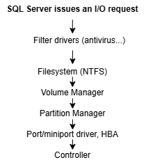
The 8 data files show nearly identical latencies and write counts (about 15.8 M each). The tempdb round-robin allocation works perfectly. This is not a hotspot, not a single bad file. The whole volume is affected.
The volume D is local to each cluster node. It is not a shared disk (not on the storage array).
Slow media or queuing?The DMV cannot separate service time from queue time. So we measured the service time directly at idle with WinSAT:
MeasureI/O profileResultIOPSRandom read16 KB451 MB/sAbout 28 900Sequential read64 KB1 965 MB/sSequential write64 KB964 MB/sRandom write8 KB (SQL Server page profile)394 MB/sAbout 50 500Read latency, maximum3.1 msThe media is excellent on all four access profiles. The verdict is simple: the 380 ms are queue time, not service time.
A quick calculation confirms it. The DMV counted about 128 M writes over 104 hours of uptime: about 340 writes per second on average. The volume can absorb 50,000. Average utilization: 0.7%. A volume used at 0.7% that shows 376 ms of average latency means one thing: the load is not smooth. It arrives in bursts. During a burst, thousands of I/Os pile up in the queue, each one waits behind the others and since most of the write volume is concentrated in those bursts they dominate the average.
Where the bursts come fromOn this instance, the bursts are produced by sort and hash operations that do not fit in their memory grant and spill to tempdb, mainly during data loads and some heavy analytical queries. The workload side of this story (memory grants, parallelism, NUMA topology) is covered in this blog : https://www.dbi-services.com/blog/wait-stats-and-sub-numa-clustering/
In this post, we follow the storage path only: whatever the workload does, a burst of writes should not cost 380 ms per I/O on a volume this fast.
The invisible layerWhen SQL Server writes a page to tempdb, the write goes through this chain:
SQL Server > Windows/NTFS > driver (SmartPqi.sys) > Smart Array controller > physical SSDs
Windows never talks to the SSDs. It talks to the RAID controller (an HPE Smart Array P408i-a) which assembles two SAS SSDs into a RAID 1 mirror and presents the result as volume D.
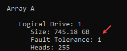
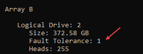
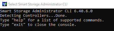
Here is the key point: every instrument used so far measures through that controller without seeing it. The DMVs measure above it. WinSAT measures above it. Only one question remains open: how is that card configured? And only one tool answers it: the Smart Storage Administrator CLI (ssacli).
 Factory settings
ctrl slot=0 show detail

   Cache Board Present: True
   Total Cache Size: 2.0
   Cache Status: Not Configured
   Battery/Capacitor Status: OK
   No-Battery Write Cache: Disabled

ctrl slot=0 ld all show detail

   Logical Drive: 2          (volume D)
      Fault Tolerance: 1     (RAID 1)
      Caching: Disabled
      LD Acceleration Method: Smart Path
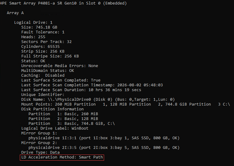
HPE SSD Smart Path is a direct I/O path: requests skip the RAID firmware stack and go straight to the SSDs. It saves a few dozen microseconds per I/O which benefits reads. But it is a per-volume switch and it is mutually exclusive with the controller cache. Smart Path is enabled by default on every SSD array (factory default). It’s reasonable for a read-oriented volume but it was never revisited for a volume hosting tempdb (one of the most write-intensive profiles there is).
The consequence: every write must be applied to both SSDs of the mirror and confirmed before it is acknowledged. There is no absorber anywhere in the chain. When a burst arrives the queue explodes.
Today (Smart Path)After (cache enabled)ReadsDirect path to the SSDsClassic path (+ a few dozen microseconds) + read cacheWritesWait for both SSDs to confirmPosted to DRAM: acknowledged in microseconds, mirror written in the background Is enabling the write cache safe?The old advice “do not enable write caching” targets a different cache: the volatile DRAM inside the disks themselves which loses acknowledged writes on power failure. That one stays disabled (Drive Write Cache Policy: Disable).
The controller cache is a different story. Microsoft’s requirement is stable media: an acknowledged write must survive a power failure. This controller qualifies through the flash-backed write cache mechanism:
- On power loss, the battery does not store any data. It powers the cache module for a few seconds just long enough for the controller to copy the DRAM content to the flash NAND chip on the module itself. Flash is non-volatile: the data survives without any power (indefinitely).
- At reboot the controller restores that data and writes it to the SSDs of the volume before accepting any new I/O.
- If the battery ever fails the controller detects it and automatically falls back to write-through.
There is a second safety belt specific to this volume: tempdb is recreated at every instance startup. Even in the worst theoretical scenario, there is no data anyone would come back for.
The possible fixThree online reversible commands:
ssacli ctrl slot=0 array B modify ssdsmartpath=disable
ssacli ctrl slot=0 ld 2 modify caching=enable
ssacli ctrl slot=0 modify cacheratio=10/90
Why cacheratio=10/90?
This setting splits the controller cache: 10% for reads, 90% for writes. It is not an exotic choice, it is the HPE factory default for a configured cache documented as the best ratio for most workloads.
Expected result: LD Acceleration Method: Controller Cache on the logical drive, Cache Status: OK on the controller.
To validate we should not rely on the cumulative DMV averages they will stay polluted by history. We should measure deltas:
- WinSAT after the change: service time should stay excellent (nothing was broken).
- sys.dm_io_virtual_file_stats deltas over a defined window covering the load phases.
- PerfMon during the load window: Avg. Disk sec/Write should stay in single digits at the peak of a burst and the queue should drain between bursts.
One expectation to set correctly: the cache absorbs bursts but it does not add throughput. All the bytes still land on the same two SSDs.
Note: these commands have not been implemented. They are proposals only. The change must be reviewed, validated and scheduled by the customer before any implementation.
Local tempdb volumes on FCI nodes: a good ideaPlacing tempdb on a local volume in a Failover Cluster Instance is supported since SQL Server 2012 and it is a good design: tempdb is recreated at startup so there is nothing to fail over. It offloads the shared storage and local SSDs deliver excellent performance for one of the hottest write profiles of the instance (our measurements above prove it).
But this choice turns storage health into a per-node responsibility:
- Check the RAID controller configuration on every node. The passive node most likely carries the same factory default. After a failover the problem would silently come back.
- Monitor Battery/Capacitor Status. A dead battery silently disables the write cache and brings the symptom back.
The architecture is right. It just makes your RAID controller part of your database health check.
Thank you. Amine Haloui
L’article When tempdb write latency points below SQL Server est apparu en premier sur dbi Blog.
Elastic Observability for Application Servers: From Monitoring to Troubleshooting Intelligence
Application servers such as WebLogic, JBoss EAP, WildFly, Tomcat, and WebSphere still run critical business applications in many enterprise environments.
However, they are often monitored like basic infrastructure components: CPU, memory, disk, process status, and sometimes port availability. This is useful, but it is not enough.

An application server can be up, the JVM can be running, and the port can respond, while users are already experiencing slow response times, blocked transactions, JDBC pool saturation, session issues, or intermittent application errors.
This is where observability brings real value. The objective is not only to know whether the server is alive. The objective is to understand how the application behaves, where it is degraded, and what needs to be fixed first.
Application servers are not just Java processes
A common mistake is to monitor application servers as if they were simple JVMs.
In reality, an application server is an execution platform. It manages applications, HTTP requests, sessions, datasources, connection pools, transactions, security, messaging, classloading, thread pools, integrations, and sometimes clustering.
When an incident happens, the root cause is rarely visible from CPU and memory alone.
A production issue can come from:
- a saturated JDBC pool,
- slow database queries,
- blocked or waiting threads,
- excessive garbage collection,
- a failing backend service,
- too many HTTP sessions,
- deployment-related errors,
- authentication or authorization failures,
- JMS queue backlog.
Traditional monitoring can tell us that something is wrong. But it often cannot explain why.
This is the gap Elastic Observability can help to close.
Elastic Observability brings together logs, metrics, traces, and application performance data in a unified platform. Elastic documents its observability solution as combining logs, metrics, application traces, user experience data, and synthetic monitoring in order to provide visibility across applications and infrastructure.
For application servers, this matters because troubleshooting is rarely based on one signal. A slow application transaction may require looking at the HTTP request, Java method execution, database call, connection pool behavior, JVM metrics, and server logs at the same time.
The real problem is fragmented troubleshootingIn many middleware environments, the data already exists but it is fragmented.
Logs are on one server. JVM metrics are in another tool. Thread dumps are collected manually. Database metrics are owned by another team. Application errors are visible only to developers. Infrastructure alerts are managed by operations. APM, if present, may not be correlated with platform logs.
During an incident, teams lose time switching between tools, comparing timestamps, grepping logs, opening server consoles, requesting database checks, and trying to reconstruct the sequence of events manually.
This is especially true for application servers, because they sit between multiple domains:
- application code,
- JVM configuration,
- database,
- messaging,
- identity provider,
- network,
- external APIs,
- container or VM platform.
The application server is often where the symptoms appear, but not always where the root cause is.
A typical example is a slow application. The server is up. CPU is normal. Memory is acceptable. But users complain.
Without observability, the investigation may start with generic checks: server status, JVM memory, recent logs, database availability, thread dumps, and maybe application team escalation.
With proper observability, the investigation can start from the user-facing symptom:
- Which endpoint is slow?
- Since when?
- Is it all users or only one application flow?
- Is the latency inside the Java application?
- Is it caused by a database call?
- Is the JDBC pool waiting?
- Is an external HTTP call slow?
- Did errors increase after a deployment?
- Are logs showing the same transaction or correlation ID?
Elastic APM is designed to collect performance information such as response times, database queries, cache calls, external HTTP requests, and related application behavior, helping to identify performance issues more quickly.
That changes the troubleshooting model. Instead of starting from the server and searching for a symptom, teams can start from the degraded service and follow the evidence.
Elastic does not replace middleware expertise, it amplifies itElastic Observability is not magic, and it does not remove the need for application server expertise. An expert still needs to understand what matters in WebLogic, JBoss EAP, WildFly, Tomcat, or WebSphere.
The value of Elastic is to make this expertise operational.
Elastic supports both its own APM agents and OpenTelemetry-based collection. Elastic documentation states that OpenTelemetry can be used to collect application performance data in Elastic APM across serverless, self-managed, and hybrid deployments. This is important for enterprise environments because you may not want to lock instrumentation strategy to a single vendor-specific approach.
In any case, a serious observability implementation should therefore start with an assessment, not with agent installation only.
For application servers, I would typically define:
- which applications are critical,
- which logs must be collected,
- which JVM and OS metrics are required,
- which application transactions need tracing,
- whether APM agent or OpenTelemetry is the best option,
- which technical indicators matter: response time, error rate, GC, threads, JDBC pool, JMS backlog, deployment events,
- which business indicators matter: failed orders, failed logins, slow reports, blocked workflows,
- which alerts are useful and which ones will create noise.
The goal is not to collect everything. The goal is to collect the right signals and correlate them.
ConclusionApplication servers remain critical in enterprise IT, but traditional monitoring is no longer enough. Knowing that a JVM is running, CPU and memory are normal, or a port is open does not explain where a performance issue actually starts.
For platforms such as WebLogic, JBoss EAP, WildFly, Tomcat, and WebSphere, real observability comes from correlating logs, metrics, traces, and application behavior.
Elastic Observability provides this visibility, helping teams move from basic monitoring to faster and more effective troubleshooting.
The real value, however, comes from combining the technology with the right expertise. Our teams bring together strong Elastic, application-server, and database expertise, enabling us to implement observability solutions that collect the right signals, provide meaningful insights, and accelerate root cause analysis.
Ultimately, observability is not about dashboards. It is about reducing blind spots, shortening incident resolution, and giving teams a shared view of production reality.
L’article Elastic Observability for Application Servers: From Monitoring to Troubleshooting Intelligence est apparu en premier sur dbi Blog.
DB2 SQL1598N Licensing Error When Upgrading GoldenGate
While upgrading GoldenGate to 26ai for a DB2 z/OS source, I had to update the IBM Data Server Driver for ODBC and CLI (CLI Driver, in short) alongside it. Since I realized that DB2 driver know-how was rare in companies, I figured it would be worth writing a blog about the topic.
In this GoldenGate upgrade, the previous driver was version 11.1 and the target version was 12.1. After installing the new driver, db2cli execsql commands that previously worked started failing with the following error:
db2cli execsql -db <database_alias> -user <username> -passwd <password> \
  -inputsql /home/oracle/input.sql
Where /home/oracle/input.sql just contains a trivial test query:
select 1 from sysibm.sysdummy1;
The sysibm.sysdummy1 table is DB2’s equivalent of Oracle’s DUAL, so this is about the simplest query you can run to check connectivity. It failed with the following error:
SQLError: 1 = 0 (SQL_SUCCESS)
SQLGetDiagRec: SQLState : 42968
NativeError : -1598
DiagMsg: [IBM][CLI Driver] SQL1598N An attempt to connect to the database server failed because of a licensing problem. SQLSTATE=42968
SQL1598N means the DB2 client does not have a valid license to connect to this database. The CLI driver loaded fine. But when it tried to establish an authenticated connection the server rejected it on licensing grounds.
This is distinct from a connection failure or an authentication failure.
Root causeIt might not be obvious for Oracle-accustomed DBAs, but the DB2 CLI Driver does not ship with a license file for connecting to DB2 for z/OS. A separate license file named db2consv_zs.lic must be placed manually in the clidriver/license/ directory of the driver installation.
The critical point is that the license file is version-specific and cannot be reused across driver versions. The license file that worked with driver 11.1 is not valid for driver 12.1. After upgrading the driver, the new installation directory does not contain the license file in the license/ folder, and copying the old license file into it will not resolve the error.
The error was reproducible every time the same command was run against the new driver. For reference, a successful run against a properly licensed driver returns:
FetchAll: Columns: 1
1
1
FetchAll: 1 rows fetched.
It is important to keep in mind that the license file belongs in the license/ subdirectory of the CLI driver installation. With CLI driver 11.1, the path looked like:
/opt/ibm/db2_odbc_cli_11_1/clidriver/license/db2consv_zs.lic
After upgrading to 12.1, the new driver has its own separate installation directory with its own license/ subdirectory. Placing the old 11.1 license file there will not work – the file is tied to the driver version.
Since the old file is unusable, you must obtain a new license file matching the installed driver version from IBM. Essentially, you have two options here:
- Contact your DB2 engineers: if someone on the team manages IBM software licenses, they should be able to provide the correct
db2consv_zs.licfor the version you installed. - Open a case with IBM customer support: IBM will provide the appropriate license file for the new driver version.
Once you have the correct file, place it in the clidriver/license/ directory of the new driver installation and retry the same db2cli execsql command given above. No restart is required.
DB2 CLI drivers are not that complicated to use and to debug. However, there are a few fundamentals that GoldenGate administrators should know before attempting a migration. Renewing the license file is one of them.
L’article DB2 SQL1598N Licensing Error When Upgrading GoldenGate est apparu en premier sur dbi Blog.
SQL Server vs MongoDB: When the cloud is your adversary (Always Encrypted vs Queryable Encryption)
When a company still refuses to put its sensitive data in the cloud, the reason usually isn’t cost or performance: it’s data sovereignty. In the cloud, someone else is the administrator of the machine; therefore the provider can, in theory, read the data files, see the data being used in memory, or read the backups. The threat model is no longer the external attacker but the privileged insider hosting the database.
As covered previously on my blog Beyond TDE and TLS: Bridging the Data Security Governance Gap in Lower Environments, various encryption methods can protect you. For example, TLS protects data in transit and TDE protects it at rest, but as soon as the engine runs a query, it handles plaintext in memory. So there are three states to protect: at-rest, in-transit, in-use. The gap this article focuses on is the last one.
That is exactly what Always Encrypted (SQL Server) and Queryable Encryption (MongoDB) target. The common principle: encryption and decryption happen client-side, in the driver; the keys never reach the engine. The data stays encrypted at rest, in transit, and during processing. The DBA, the cloud operator, the hypervisor admin: all of them see only cyphertext.
That leaves one question: if the engine sees only cyphertext, how does it answer a WHERE condition? Both database engines do answer it, but through different technical means.
To demonstrate all this, let’s start by creating a table with two columns, Salary and Department, encrypted deterministically on one side and randomized on the other:
DROP TABLE IF EXISTS dbo.Employees;
CREATE TABLE dbo.Employees (
  Id         INT IDENTITY(1,1) PRIMARY KEY,
  LastName   NVARCHAR(50) COLLATE Latin1_General_BIN2 NOT NULL,
  FirstName  NVARCHAR(50) COLLATE Latin1_General_BIN2 NOT NULL,
  DeptDet    NVARCHAR(30) COLLATE Latin1_General_BIN2 NOT NULL, -- will be DETERMINISTIC
  DeptRand   NVARCHAR(30) COLLATE Latin1_General_BIN2 NOT NULL, -- will be RANDOMIZED
  SalaryDet  INT NOT NULL, -- will be DETERMINISTIC
  SalaryRand INT NOT NULL  -- will be RANDOMIZED
);
GO

INSERT INTO dbo.Employees (LastName, FirstName, DeptDet, DeptRand, SalaryDet, SalaryRand) VALUES
('Martin',  'Alice', 'Sales', 'Sales', 55000, 55000),
('Dubois',  'Bob',   'Sales', 'Sales', 48000, 48000),
('Bernard', 'Chloe', 'Sales', 'Sales', 52000, 52000),
('Petit',   'David', 'IT',    'IT',    72000, 72000),
('Durand',  'Emma',  'IT',    'IT',    68000, 68000);
Five rows: three Sales, two IT. The BIN2 collation is required by Always Encrypted (link to documentation), and the master key lives outside the database (Key Vault, certificate store, or HSM).
Column encryption isn’t done in T-SQL, because the engine doesn’t have the keys. It’s driven from the client (here in PowerShell), declaring for each value a deterministic column and its randomized twin:
Import-Module SqlServer -MinimumVersion 22.0.59
$sqlConnectionString = "Data Source=.\LAB2025;Initial Catalog=AEDEMO;Integrated Security=True;Encrypt=False;Trust Server Certificate=False"
$smoDatabase = Get-SqlDatabase -ConnectionString $sqlConnectionString

$encryptionChanges  = @()
$encryptionChanges += New-SqlColumnEncryptionSettings -ColumnName dbo.Employees.DeptDet    -EncryptionType Deterministic -EncryptionKey "CEK1"
$encryptionChanges += New-SqlColumnEncryptionSettings -ColumnName dbo.Employees.DeptRand   -EncryptionType Randomized    -EncryptionKey "CEK1"
$encryptionChanges += New-SqlColumnEncryptionSettings -ColumnName dbo.Employees.SalaryDet  -EncryptionType Deterministic -EncryptionKey "CEK1"
$encryptionChanges += New-SqlColumnEncryptionSettings -ColumnName dbo.Employees.SalaryRand -EncryptionType Randomized    -EncryptionKey "CEK1"

Set-SqlColumnEncryption -ColumnEncryptionSettings $encryptionChanges -InputObject $smoDatabase
In this example, I’m working on my 2025 SQL Server instance, on the AEDEMO database, using the column encryption key CEK1 I created beforehand (itself protected by a column master key stored outside the database).
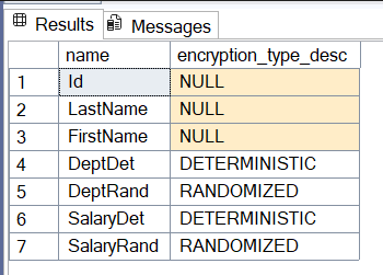
We check that the engine sees the right type per column:
SELECT c.name, c.encryption_type_desc
FROM sys.columns c
WHERE c.object_id = OBJECT_ID('dbo.Employees');
The deterministic mechanism works like this: same plaintext, same cyphertext (an injective function). On an Always Encrypted-enabled connection with Parameterization for Always Encrypted and parameters for the predicates (never literals), equality works:
DECLARE @d NVARCHAR(30) = 'Sales';
SELECT DeptDet AS Enc, COUNT(*) FROM dbo.Employees WHERE DeptDet = @d
GROUP BY DeptDet;
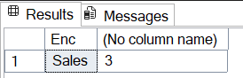
The driver encrypts @d with the same key, the server finds the encrypted values that are identical to the parameter, and the result is correct.
You pay for it in three ways…
First weakness: deterministic encryption can cause a data leak. You don’t need the keys to see it. Just connect without Always Encrypted and read the table: the encrypted columns come out as raw binary.
SELECT FirstName, DeptDet, DeptRand FROM dbo.Employees;

Look at the DeptDet column: Alice, Bob, and Chloe share exactly the same blob, and David and Emma share another. Two distinct values across five rows. The adversary doesn’t know what 0x012536… means, but reads the structure: two departments, one with three people, the other with two, and who goes with whom. The DeptRand column, on the other hand, shows five all-different blobs: nothing to read.
It’s harmless on five rows; it isn’t on a real table. On a low-cardinality column (region, sex, status), the distribution of blobs can be compared to a known distribution, and frequency analysis often reconstructs the plaintext. Microsoft’s documentation puts it bluntly: an unauthorized user can guess information by examining patterns, especially when the set of possible values is small.
Second weakness: randomized encryption blocks every query. With randomized encryption, the driver adds a fresh random value to each cell before encrypting, so the same input produces a different cyphertext every time. Therefore, the leak is gone but so is the query:
DECLARE @d NVARCHAR(30) = 'Sales';
SELECT DeptRand AS Enc, COUNT(*) FROM dbo.Employees WHERE DeptRand = @d
GROUP BY DeptRand;
Msg 33277, Level 16, State 2, Line 6
Encryption scheme mismatch for columns/variables ‘DeptRand’, ‘@d’. The
encryption scheme for the columns/variables is (encryption_type =
‘RANDOMIZED’, …) and the expression near line ‘6’ expects it to be
DETERMINISTIC, or RANDOMIZED, a BIN2 collation for string data types,
and an enclave-enabled column encryption key, or PLAINTEXT.
The server can no longer compare, since the same plaintext produces a different cyphertext on every row. We gained confidentiality and lost the query. It’s all or nothing.
Third weakness: no range, even with deterministic. Byte equality says nothing about order:
DECLARE @s INT = 55000;
SELECT FirstName FROM dbo.Employees WHERE SalaryDet < @s;
WHERE SalaryDet < @s fails even though the column is deterministic. Sorting, BETWEEN, LIKE: out of reach for Always Encrypted alone.
The verdict is clear: bare Always Encrypted means equality, or nothing (=, IN, GROUP BY, and DISTINCT supported).
MongoDB: queryability lives in a protocolMongoDB’s Queryable Encryption makes optimal use of randomized encryption. On the server side, everything is Randomized-encrypted, as the documentation explains: the server has no knowledge of the data it processes. The encrypted view (a client connected without the keys) confirms it: even the three Sales employees come out with all-different BinData.
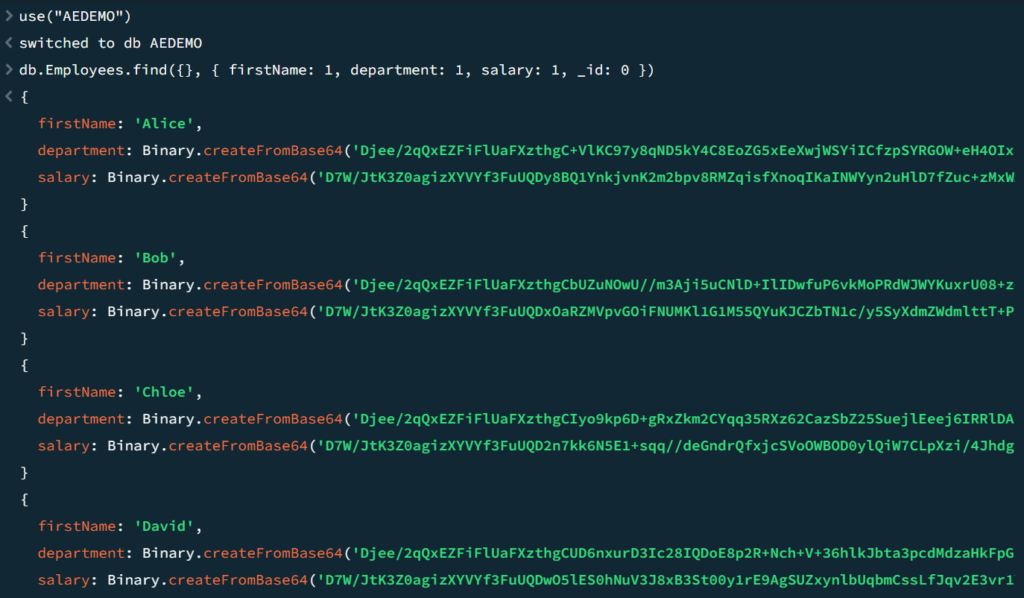
No frequency leak, unlike SQL Server’s deterministic encryption. With the keys, the same find returns the plaintext:
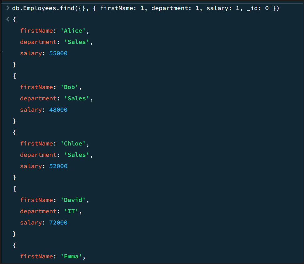
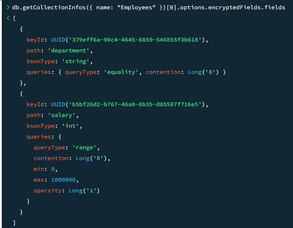
The technical mechanism behind this lies in the collection’s declaration. Each encrypted field carries a queryType, its parameters, and a distinct key (keyId), one Data Encryption Key per field, which is mandatory:
And queries with equality tests, range, and even equality on a field declared as range all work:
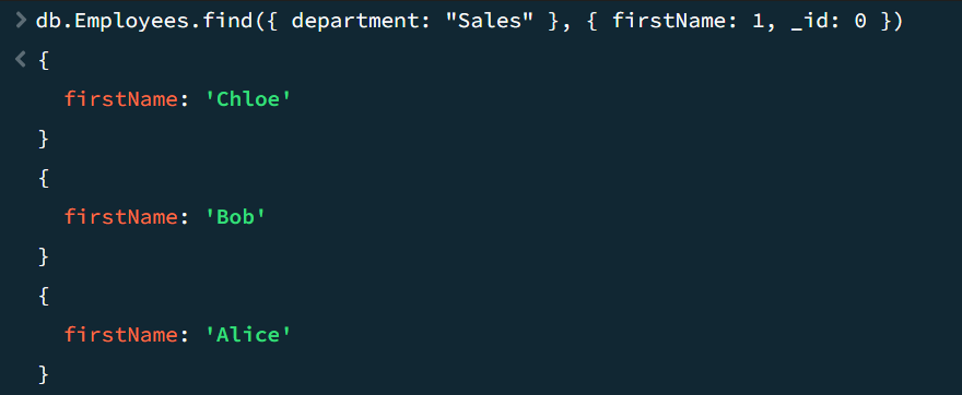
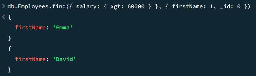

On the server side, MongoDB then maintains encrypted index structures, and for each query the driver generates cryptographic tokens that the server checks against those structures without ever seeing the plaintext. This is a searchable encryption scheme. Range is available in GA, with no special hardware.
The real difference comes down to one thing: the driverOn the SQL Server side, the driver’s work stays thin: it encrypts the parameters, rewrites the query, decrypts the results. Queryability itself is already carried by the cyphertext; the driver doesn’t have to handle it. On the MongoDB side, the driver carries the whole protocol: it generates the tokens checked against the encrypted indexes.
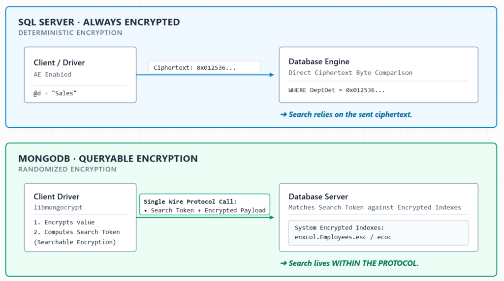
Once the collection is in place, find({ department: "Sales" }) is written like a normal query and the driver handles the encryption on its own. Each encrypted field needs its own key (Data Encryption Key). The master key must be pinned, otherwise orphaned keys return an HMAC validation failure error. And the encryption API is only available from a client created as encrypted, so not from a standard Compass connection, for example.
This is where secure enclaves come in. The engine delegates the computation to an enclave: a protected memory region where the data is decrypted and processed in the clear, out of reach, including from the machine’s administrator. This is what unlocks range, LIKE, sorting, and in-place encryption: inside the enclave the server no longer compares encrypted bytes, it works on the plaintext. This gain has a price. It requires compatible hardware or secure virtualization, an attestation service to deploy and maintain, and keys configured for the enclave, which noticeably increases architectural complexity compared with classic Always Encrypted.
But it also changes the nature of the trust. Queryable Encryption rests on a cryptographic guarantee: the server cannot read, it’s a mathematical property. Enclaves rest on a hardware guarantee: you trust the CPU, and its attestation, to isolate the protected region.
There remains a third path, often mentioned: homomorphic encryption (FHE), which computes directly on the cyphertext without ever decrypting it. Elegant on paper, but out of the game for database search: the computational cost is massive and response time collapses as the volume grows. So the practical choice really does play out between the two worlds described here.
L’article SQL Server vs MongoDB: When the cloud is your adversary (Always Encrypted vs Queryable Encryption) est apparu en premier sur dbi Blog.
Wait stats and Sub-NUMA clustering
During a healthcheck at a client’s site, we collected performance data from a SQL Server 2019 Enterprise instance hosting a BI / data warehouse workload. Two lines in the wait statistics report immediately caught the eye: hundreds of hours of parallelism waits accumulated in only 11 days of uptime.
Here are the questions that arise
- Can a wait type really account for more than 100% of server uptime?
- Are these values a problem in themselves?
- What do they tell us about the configuration of the instance?
The waits themselves were not the problem. But they pointed us to a BIOS option (Sub-NUMA Clustering) that was silently reshaping the entire NUMA topology of the server and putting it in conflict with the MAXDOP configuration.
This post is the story of that investigation: from the wait statistics to the BIOS, step by step.
Unusual wait statisticsThe collected data
The instance had been up for about 11 days (roughly 273 hours). The two top wait types were:
761 hours is almost 32 days. How can a server accumulate 32 days of waits in 11 days of wall-clock time?
Reading percentages above 100%
Wait statistics are cumulated across all threads that are waiting at the same time. A waiting thread is in the SUSPENDED state: it does not occupy a scheduler, so the number of simultaneous waiters is not limited by the number of CPUs. It is only limited by the worker thread pool (704 workers on this instance).
A simple example: 16 threads, each waiting for one hour during one hour of wall-clock time, produce 16 hours of wait time for 1 hour of uptime. That is 1600%.
This gives us the only robust way to read these percentages: divide by 100 to get the average number of threads simultaneously waiting on that wait type.
- CXCONSUMER: 761.91 h / 273 h ≈ 2.79 → about 2.8 threads permanently waiting
- CXPACKET: 657.78 h / 273 h ≈ 2.41 → about 2.4 threads permanently waiting
On a server that can host 704 workers, 2.5 permanent waiters is not an alarming number.
CXPACKET and CXCONSUMER
Both wait types belong to parallel query execution. A parallel plan splits its work into branches and the branches synchronize at exchange operators.
- CXCONSUMER: the consumer side of an exchange is simply waiting for the producers to deliver rows. This is the structural, unavoidable wait of any parallel plan. It is considered benign.
- CXPACKET: a thread has finished its share of the work and waits for slower branches at the synchronization point. This is the potentially actionable signal: it reveals an imbalance between the branches of the plan.
An analogy: in a factory, CXCONSUMER is a workstation waiting for parts to arrive (normal), CXPACKET is a workstation that has finished its batch and waits for a slower colleague (an imbalance worth examining).
Are these values abnormal, then?
Look at the averages again: 0.00 ms and 1.00 ms per wait. 657.78 hours at 1 ms average means roughly 2.4 billion individual waits. These counters do not describe long blockings, they describe the normal tick-tock of exchange operators in a heavily parallel workload. A server suffering from severe skew would show averages of tens of milliseconds.
The healthcheck tool itself says it in its own message: “Usually a cost threshold for parallelism / MAXDOP tuning issue rather than a problem in itself.” The line is an inventory entry (any wait above 10% of uptime gets reported), not an alarm.
So why did these two lines matter? Not because of their height because of their rank. CXCONSUMER and CXPACKET were number 1 and number 2 of the entire wait inventory, ahead of everything else. Their rank designated parallelism as the dominant workload of this instance and therefore its configuration as the first thing to confront with the topology.
The instance configuration
SELECT [name], value_in_use
FROM sys.configurations
WHERE [name] IN (N'max degree of parallelism', N'cost threshold for parallelism'); - Cost threshold for parallelism: 50, correctly raised from the default of 5. This setting decides which queries are allowed to go parallel (those whose estimated cost exceeds the threshold).
- MAXDOP: 8, this setting decides how wide: the maximum number of worker threads per parallel branch.
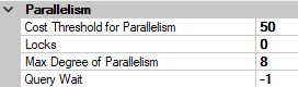
MAXDOP 8 is a perfectly reasonable value in isolation. The problem only appears when we look at the topology.
The topology
SELECT cpu_count, hyperthread_ratio, socket_count, cores_per_socket,
numa_node_count, softnuma_configuration_desc
FROM sys.dm_os_sys_info; 
Two sockets. Four NUMA nodes. That is the anomaly this whole post is about.
From the anomaly to the root causeOn modern processors, there is no central memory controller shared by all cores. Each processor package has its own memory controllers with its own RAM modules attached to them. Such a group (cores + memory controllers + local RAM) is a NUMA node.
When a core reads an address that lives in its own node’s RAM: direct path, fast. When it reads an address that lives in another node’s RAM: the request crosses the interconnect, with roughly 1.5 to 2 times the latency. That is the meaning of the name: Non-Uniform Memory Access. The cost of a memory access depends on the physical distance between the core that asks and the RAM module that answers.
The natural NUMA boundary is therefore the socket: one socket = its memory controllers = its local RAM = one NUMA node.
Here we have 4 nodes for 2 sockets: 2 nodes per socket. Only three mechanisms can produce that:
Cross-checking with the hardware
The server is a physical HPE ProLiant DL380 Gen10 with 2 × Intel Xeon Gold 6244 (8 cores / 16 threads each, 3.60 GHz base) and 384 GB of RAM (12 × 32 GB, balanced across the memory channels).
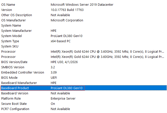
Windows server shows “8 Core(s), 8 Logical Processor(s)” per socket, and Task Manager shows Cores: 16 = Logical processors: 16. Hyper-threading is disabled: 16 physical cores, one logical processor per core. This matters for the rest of the post, because Microsoft’s MAXDOP recommendations are expressed in logical processors per node.
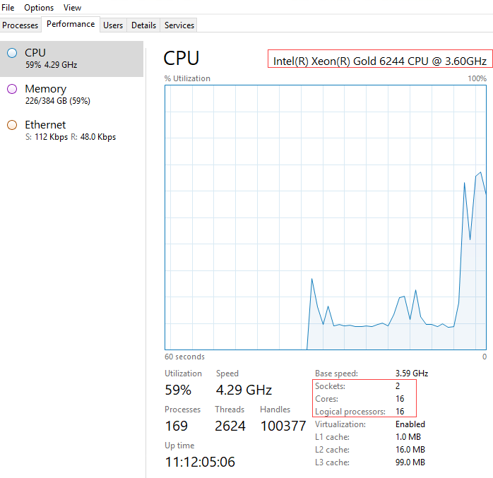
A corroborating detail: Task Manager reports L3 cache = 99.0 MB. The Gold 6244 has 24.75 MB of L3 per socket, so the server has 49.5 MB but 99.0 = 4 × 24.75. Windows counts the socket’s L3 once per NUMA node it is presented with. The only wrong line in the cache arithmetic is exactly the one that depends on NUMA counting.
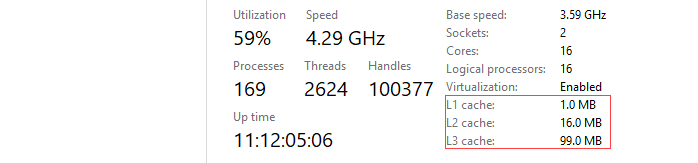 What Sub-NUMA Clustering is
Our socket contains 8 cores, 6 memory channels and a shared L3 cache connected by an internal mesh. Sub-NUMA Clustering (SNC) is a BIOS option that cuts this socket into two domains, each with 4 cores, 3 memory channels and its half of the L3 affinity and presents each half as a full NUMA node to the operating system.
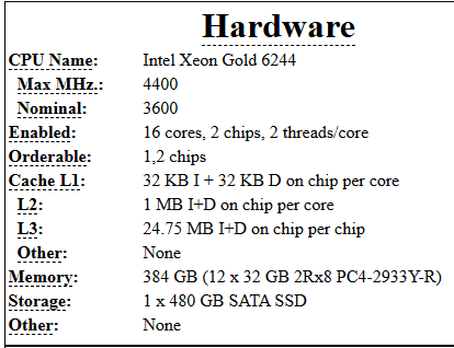
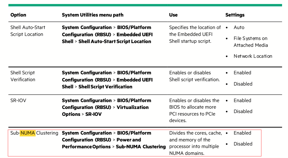
Two sockets × SNC = 4 NUMA nodes of 4 logical processors and about 96 GB of RAM each. Exactly what our DMVs show.
Why does this option exist? Because for some workloads it helps. A public SPEC CPU2017 result published by Dell on the equivalent platform (PowerEdge R640, same 2 × Xeon Gold 6244, same 384 GB in 12 × 32 GB) is instructive on this point the BIOS notes literally list “Sub NUMA Cluster enabled” and the published numactl output shows the resulting topology:
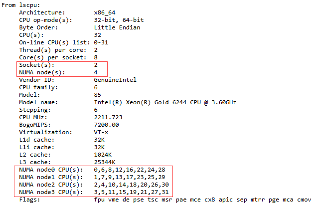

Reference : https://www.spec.org/cpu2017/results/res2019q2/cpu2017-20190429-12798.html
What SNC makes SQLOS build
At startup, SQLOS mirrors the presented topology: one memory node and one group of schedulers per NUMA node. On this server: 4 groups of 4 schedulers and the decisive point the buffer pool is partitioned across the 4 nodes. With max server memory at 210 GB, each node manages roughly 52 GB, and a cached data page physically lives in the RAM of one node.
The mechanics then the correctionsNow we can close the loop with Part 1:
- SNC (BIOS) cuts 2 sockets into 4 NUMA nodes of 4 logical processors.
- MAXDOP is 8 and a node only offers 4 schedulers: every parallel query spans two nodes by construction at every execution.
- The workers on the remote node access non-local memory. This cost is mostly invisible in the wait statistics a thread reading remote memory is RUNNING, not waiting. The direct cost hides in queries that simply run slower.
- Only the indirect effect surfaces: asymmetric memory distances desynchronize the branches, the fast workers finish their packets and wait for the slow ones at the exchanges and that spills into CXPACKET.
- The placement follows the load of the moment, so the same query can have different costs from one execution to the next. SNC does not only add cost it adds variance.
Why MAXDOP 4 alone is not the fix
Capping MAXDOP at 4 confines each query’s workers to a single node. That offers two things: the working memory (memory grants, hash tables, sort runs, exchange buffers) becomes local and all branches advance at the same speed and nobody waits for a remote colleague anymore.
But it does not buy data locality. A buffer pool page is allocated on the node of the worker that read it from disk potentially days ago for another query on another node and it never migrates afterwards. With 4 nodes, a query confined to node 2 finds on average only about 25% of the already-cached pages locally. And MAXDOP 4 also halves the width of every query on a data warehouse that lives on parallelism. MAXDOP 4 is the bandage. The correction is the topology itself.
Microsoft’s recommendations Configuration MAXDOP recommendation Single NUMA node, ≤ 8 logical processors ≤ number of logical processors Single NUMA node, > 8 logical processors 8 Multiple NUMA nodes, ≤ 16 logical processors per node ≤ number of logical processors per node Multiple NUMA nodes, > 16 logical processors per node Half the logical processors per node, max 16Our server sits on the third line in every scenario:
Scenario Topology MAXDOP recommendation Today (SNC enabled) 4 nodes × 4 logical processors ≤ 4 (currently 8: non-compliant) SNC disabled 2 nodes × 8 logical processors ≤ 8 → the current setting becomes compliantCurrent (SNC enabled) :
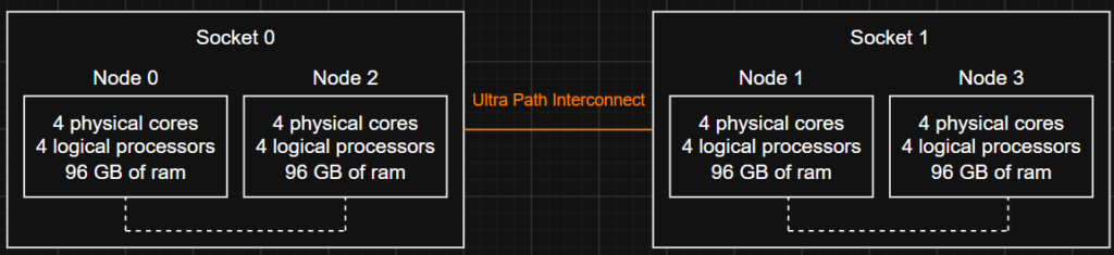
After (with SNC disabled) :
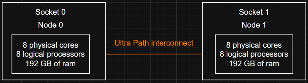
The possible two corrections:
Short term (online, reversible, no restart): MAXDOP = 4. It confines each query to one node as the server is presented today. It is a transitional measure not the target state.
EXEC sp_configure 'max degree of parallelism', 4;
RECONFIGURE;
Root-cause correction (through a maintenance window): disable SNC in the BIOS. On an HPE Gen10, the option lives in:
System Configuration > BIOS/Platform Configuration (RBSU) > Power and Performance Options > Sub-NUMA Clustering > Disabled
It looks like that:
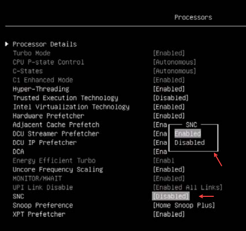
Reference : https://lenovopress.lenovo.com/lp1499.pdf
ConclusionThe wait statistics never proved anything in this story and that is the point. Values above 100% of uptime are normal (they cumulate across all simultaneous waiters), the averages were small and CXCONSUMER is benign by nature. What the two lines provided was a characterization: normalized by uptime, they showed about 2.5 threads permanently synchronizing exchanges and this instance lives on parallelism. Their rank designated parallelism as the dominant workload and therefore its configuration as the first thing to confront with the topology.
Thank you. Amine Haloui
L’article Wait stats and Sub-NUMA clustering est apparu en premier sur dbi Blog.
MongoDB OIDC Authentication with Okta
Since version 7.0.11, MongoDB natively supports OpenID Connect (OIDC) authentication. This move was part of MongoDB’s cloud strategy, since cloud environments use OIDC a lot for authentication and authorization. In version 8.0, MongoDB deprecated LDAP authentication and authorization, making it clear that OIDC is the future for MongoDB authentication. In this blog, I will present how to set up OIDC authentication for MongoDB in a self-managed environment with Okta.
What is OpenID Connect (OIDC) ?OpenID Connect (OIDC) is an authentication protocol built on top of the OAuth 2.0 framework. It allows clients (like mongosh) to check the identity of the user based on the authentication performed by an authorization server (like Okta). It also provides a standardized way of obtaining user profile information, resolving the authorization part of the connection.
MongoDB supports OIDC authentication for both:
- Users : Workforce Identity Federation
- Applications : Workload Identity Federation
In this blog, I will focus on the first use case.
PrerequisitesBefore setting up OIDC authentication for MongoDB, you will need the following:
- MongoDB Enterprise Edition. OIDC authentication is only available in the Enterprise Edition of MongoDB. Alternatively, you can use Percona Server for MongoDB, which also supports OIDC authentication.
- Version 7.0.11 or later of MongoDB.
- A working Okta tenant. A 30-day trial can be obtained here.
Throughout this blog, I will use very generic names (dbiapp, dbiauth, etc.) to make sure you are not missing on configuration aspects. Some of these names will be used when configuring OIDC in MongoDB.
Configure OIDC in Okta Create an application in OktaStart by creating an application in Okta. From the Admin Console (available at https://trial-1234567-admin.okta.com/admin/dashboard), navigate to Applications > Applications and click on Create App Integration. Then, select OIDC – OpenID Connect as the sign-in method and Native as the application type. Click on Next.
In the application configuration screen, fill in an application name (mine will be called dbiapp), and select Grant types among these three choices:
- Authorization Code: Activated by default, cannot be deactivated.
- Device Authorization: Required if you have no browser access when using
mongosh. The shell will display a URL with which you will authenticate. - Refresh Token: If enabled, the MongoDB driver caches the refresh token and renews the access token when it expires.
Then fill in the Sign-in redirect URIs with the following URL : http://localhost:27097/redirect

Finally, in the Assignments section, you can choose between multiple Controlled access options:
- Allow everyone in your organization to access
- Limit access to selected groups
- Skip group assignment for now
In this blog, I will choose Allow everyone in your organization to access. In production environments, you might choose something else. Make sure Enable immediate access with Federation Broker Mode is enabled, and click on Save.
You should now land on the newly created application page. Copy the Client ID displayed on the screen, you will need it later.
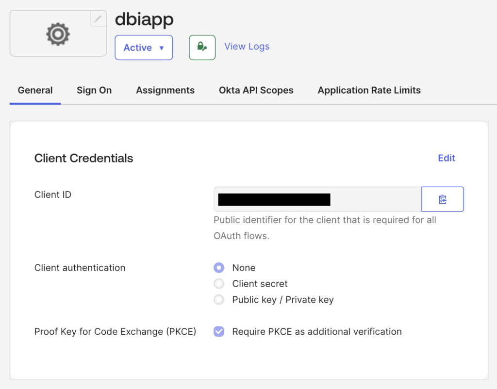
In the navigation panel, click on Security > API, and Add Authorization Server.
Choose a name for the Authorization Server (mine will be named dbiauth), and paste the Client ID retrieved earlier in the Audience field.
From the newly created authorization server, copy the Issuer Metadata URI, from https until .well-known (excluded). You should have something like https://trial-1234567.okta.com/oauth2/aus27qkm93wcRptbz412.
Staying on the authorization server summary, click on the Claims tab, and then on Add Claim.
You can choose any name for the claim. I will call it dbiclaim. The rest of the claim should be configured as follows, with the Filter set to Matches regex, using .* as filter.
WARNING: Make sure the filter is .*, not *.* or *. ! Otherwise, it could lead to MongoServerError: Authentication failed. errors.
Now, in the Access Policies tab of the authorization server, click on Add Policy.
You can choose the name of the policy that you want (mine is called dbipolicy), and you must add a Description. Set Assign to to All clients.
After creating the policy, click on Add rule.
This is the part where you should be customizing the rule based on your internal security policies. I will name my rule dbirule, and keep everything default except for the Refresh token lifetime, which is set to Unlimited.
If you already use Okta, you should have existing groups and users. But for the purpose of the blog, let’s create a group and a user. Navigate on the left to Directory > Groups, and click on Add Group.
MongoDB names the group OIDC, without stating whether it is the only name supported or not. But you can choose your own name. I will call the group dbigroup.
After creating the group, add a user in the Directory > People section, clicking on Add Person.
There are two important aspects here:
- Use an email for the Username field.
- Add the
dbigroupgroup to the Groups.
Before continuing, make sure the user is activated following the procedure received by email
Configure MongoDB for OIDC authenticationStop your MongoDB 7.0.11+ Enterprise Edition instance, and edit the configuration file by adding the following setParameter section:
authenticationMechanisms: set it toMONGODB-OIDCif you want to enable only OIDC authentication, orMONGODB-OIDC,SCRAM-SHA-256if you want to keep authentication with password for previous users.issuer: use the Issuer Metadata URI copied after creating the authorization server (https://trial-1234567.okta.com/oauth2/aus27qkm93wcRptbz412)audienceandclientId: for both fields, use the Client ID associated with the application created at the very beginning (0oa89cvj16d4WFKrX307, for instance)authNamePrefix:okta-issuerauthorizationClaim: use the name of the claim created on the authorization server. In my case, it isdbiclaim.
# Paste this at the end of your MongoDB configuration file
setParameter:
   authenticationMechanisms: "MONGODB-OIDC"
   oidcIdentityProviders: '[ {
      "issuer": "https://trial-1234567.okta.com/oauth2/aus27qkm93wcRptbz412",
      "audience": "0oa89cvj16d4WFKrX307",
      "authNamePrefix": "okta-issuer",
      "authorizationClaim": "dbiclaim",
      "clientId": "0oa89cvj16d4WFKrX307"
   } ]'
After changing the configuration file, you can restart your MongoDB instance. If security.authorization is not enabled yet, you should set it now and make sure you have a user able to create roles.
Log in with a privileged user to your MongoDB instance, and create a new role for OIDC authentication. The role name should be based on authNamePrefix (okta-issuer) and the group name (dbigroup). In this blog, I will create the okta-issuer/dbigroup role.
use admin
db.createRole( {
   role: "okta-issuer/dbigroup",
   privileges: [ ],
   roles: [ "readWriteAnyDatabase" ]
} )
Now, any member of the dbigroup group should be able to log in with mongosh or any other connection tool, with the following parameters:
--authenticationMechanismflag set toMONGODB-OIDC. This parameter value is the official MongoDB parameter.--oidcFlowsflag set todevice-auth. This can be used in environments wheremongoshwill not be able to launch a browser.
# Change the MONGO_URI accordingly
MONGO_URI="mongodb://127.0.0.1:27017"
mongosh "$MONGO_URI" --authenticationMechanism MONGODB-OIDC --oidcFlows=device-auth
After a few seconds, you will receive the URL to complete authentication:
mongodb@mongodb-lab-01:/home/mongodb/ [mdb02] mongosh "$MONGO_URI" --authenticationMechanism MONGODB-OIDC --oidcFlows=device-auth
Current Mongosh Log ID:	6a64a98717240b2e9d9df8a2
Connecting to:		mongodb://127.0.0.1:27017/?directConnection=true&serverSelectionTimeoutMS=2000&authMechanism=MONGODB-OIDC&appName=mongosh+2.9.2

Visit the following URL to complete authentication: https://trial-1234567.okta.com/activate
Enter the following code on that page: RQXFMWTF
Waiting...
You can now open the link given (https://trial-1234567.okta.com/activate), and it will ask for the activation code (RQXFMWTF).
Once the device is activated, the mongosh prompt will succeed:
mongodb@mongodb-lab-01:/home/mongodb/ [mdb02] mongosh "$MONGO_URI" --authenticationMechanism MONGODB-OIDC --oidcFlows=device-auth
Current Mongosh Log ID:	6a64a98717240b2e9d9df8a2
Connecting to:		mongodb://127.0.0.1:27017/?directConnection=true&serverSelectionTimeoutMS=2000&authMechanism=MONGODB-OIDC&appName=mongosh+2.9.2

Visit the following URL to complete authentication: https://trial-1234567.okta.com/activate
Enter the following code on that page: RQXFMWTF
Waiting...
Using MongoDB:		8.0.26
Using Mongosh:		2.9.2

Enterprise test>
And if you run the db.runCommand({connectionStatus:1}) command, you will see the OIDC connection information:
Enterprise test> db.runCommand({connectionStatus:1})
{
  authInfo: {
    authenticatedUsers: [ { user: 'okta-issuer/dbiblog@dbi-services.com', db: '$external' } ],
    authenticatedUserRoles: [
      { role: 'okta-issuer/Everyone', db: 'admin' },
      { role: 'okta-issuer/dbigroup', db: 'admin' },
      { role: 'readWriteAnyDatabase', db: 'admin' }
    ]
  },
  ok: 1
}If you use the MongoDB DMK, you should either adapt the msp alias or create a new msoidc alias to connect to your instances. To do so, edit the local configuration file of DMK with the dmkl alias:
# Option 1: change the msp alias
alias::msp::novar_noforce::'ms --authenticationMechanism MONGODB-OIDC --oidcFlows=device-auth'::

# Option 2: add a new msoidc alias
alias::msoidc::novar_noforce::'ms --authenticationMechanism MONGODB-OIDC --oidcFlows=device-auth'::
L’article MongoDB OIDC Authentication with Okta est apparu en premier sur dbi Blog.
Oracle: Standard Edition 2 available with 23.26.3.?
When downloading Release Update 23.26.3., I could see this:
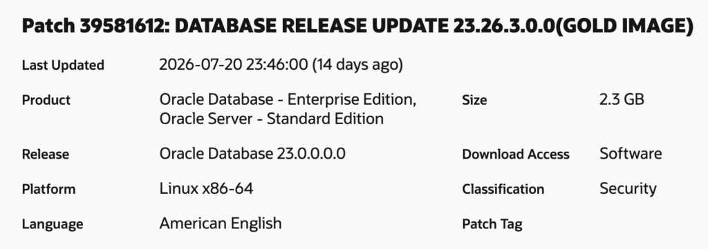
As you can see in the Product info it also has “Oracle Server – Standard Edition”. However, I haven’t found anything official yet.
I tried it and could install 23.26.3. as a Standard Edition ORACLE_HOME:
[oracle@oel10db26ai dbhome_1]$ mkdir -p /u01/app/oracle/product/26.0.0/dbhome_1
[oracle@oel10db26ai dbhome_1]$ cd /u01/app/oracle/product/26.0.0/dbhome_1
[oracle@oel10db26ai dbhome_1]$ unzip -q /tmp/p39581612_230000_Linux-x86-64.zip
[oracle@oel10db26ai dbhome_1]$ vi install/response/db_install_26ai.rsp
[oracle@oel10db26ai dbhome_1]$ cat install/response/db_install_26ai.rsp
oracle.install.responseFileVersion=/oracle/install/rspfmt_dbinstall_response_schema_v23.0.0
installOption=INSTALL_DB_SWONLY
UNIX_GROUP_NAME=oinstall
INVENTORY_LOCATION=/u01/app/oraInventory
ORACLE_HOME=/u01/app/oracle/product/26.0.0/dbhome_1
ORACLE_BASE=/u01/app/oracle
installEdition=SE2
OSDBA=oinstall
OSOPER=oinstall
OSBACKUPDBA=oinstall
OSDGDBA=oinstall
OSKMDBA=oinstall
OSRACDBA=oinstall
executeRootScript=false
dbType=GENERAL_PURPOSE
[oracle@oel10db26ai dbhome_1]$

[oracle@oel10db26ai dbhome_1]$ ./runInstaller -ignorePrereq -waitforcompletion -silent -responseFile install/response/db_install_26ai.rsp
Launching Oracle AI Database Setup Wizard...
...
[WARNING] [INS-13014] Target environment does not meet some optional requirements.
   CAUSE: Some of the optional prerequisites are not met. See logs for details. installActions2026-08-04_07-18-59PM.log.
   ACTION: Identify the list of failed prerequisite checks from the log: installActions2026-08-04_07-18-59PM.log. Then either from the log file or from installation manual find the appropriate configuration to meet the prerequisites and fix it manually.
The response file for this session can be found at:
 /u01/app/oracle/product/26.0.0/dbhome_1/install/response/db_2026-08-04_07-18-59PM.rsp

You can find the log of this install session at:
 /tmp/InstallActions2026-08-04_07-18-59PM/installActions2026-08-04_07-18-59PM.log


As a root user, run the following script(s):
	1. /u01/app/oraInventory/orainstRoot.sh
	2. /u01/app/oracle/product/26.0.0/dbhome_1/root.sh

Run /u01/app/oraInventory/orainstRoot.sh on the following nodes:
[oel10db26ai]
Run /u01/app/oracle/product/26.0.0/dbhome_1/root.sh on the following nodes:
[oel10db26ai]


Successfully Setup Software with warning(s).
Moved the install session logs to:
 /u01/app/oraInventory/logs/InstallActions2026-08-04_07-18-59PM
[oracle@oel10db26ai dbhome_1]$
After running the root-scripts I created a Database and verified that it is really a Standard Edition 2 DB:
[root@oel10db26ai ~]# mkdir /u02
[root@oel10db26ai ~]# chown oracle:oinstall /u02
[root@oel10db26ai ~]#

[oracle@oel10db26ai ~]$ mkdir /u02/oradata
[oracle@oel10db26ai ~]$
[oracle@oel10db26ai ~]$ . oraenv
ORACLE_SID = [oracle] ? dummyx
ORACLE_HOME = [/home/oracle] ? /u01/app/oracle/product/26.0.0/dbhome_1
The Oracle base has been set to /u01/app/oracle
[oracle@oel10db26ai ~]$

[oracle@oel10db26ai ~]$ export ORACLE_SID=DB26SE2
[oracle@oel10db26ai ~]$ export PDB_NAME=pdb1
[oracle@oel10db26ai ~]$ export DATA_DIR=/u02/oradata

[oracle@oel10db26ai ~]$ dbca -silent -createDatabase                                                   \
     -templateName General_Purpose.dbc                                         \
     -gdbname ${ORACLE_SID} -sid  ${ORACLE_SID} -responseFile NO_VALUE         \
     -characterSet AL32UTF8                                                    \
     -sysPassword HEllo01__01                                                 \
     -systemPassword HEllo01__01                                              \
     -createAsContainerDatabase true                                           \
     -numberOfPDBs 1                                                           \
     -pdbName ${PDB_NAME}                                                      \
     -pdbAdminPassword HEllo01__01                                            \
     -databaseType MULTIPURPOSE                                                \
     -memoryMgmtType auto_sga                                                  \
     -totalMemory 2000                                                         \
     -storageType FS                                                           \
     -datafileDestination "${DATA_DIR}"                                        \
     -redoLogFileSize 100                                                       \
     -emConfiguration NONE                                                     \
     -ignorePreReqs
...
[oracle@oel10db26ai ~]$ sqlplus / as sysdba

SQL*Plus: Release 23.26.3.0.0 - Production on Wed Aug 5 10:42:48 2026
Version 23.26.3.0.0

Copyright (c) 1982, 2026, Oracle.  All rights reserved.


Connected to:
Oracle AI Database 26ai Standard Edition 2 Release 23.26.3.0.0 - Production
Version 23.26.3.0.0

SQL> select banner from v$version;

BANNER
--------------------------------------------------------------------------------
Oracle AI Database 26ai Standard Edition 2 Release 23.26.3.0.0 - Production

SQL> show pdbs

    CON_ID CON_NAME			  OPEN MODE  RESTRICTED
---------- ------------------------------ ---------- ----------
	 2 PDB$SEED			  READ ONLY  NO
	 3 PDB1 			  READ WRITE NO
SQL> show parameter control_management_pack_access

NAME				     TYPE	 VALUE
------------------------------------ ----------- ------------------------------
control_management_pack_access	     string	 NONE
SQL>
It really seems a Standard Edition 2 DB. But let me check if it restricts me for a command not allowed in SE2:
SQL> select min(snap_id), max(snap_id) from dba_hist_snapshot;

MIN(SNAP_ID) MAX(SNAP_ID)
------------ ------------
	   1	       14

SQL> var retval number;
SQL> exec :retval:=dbms_spm.load_plans_from_awr(1,14);
BEGIN :retval:=dbms_spm.load_plans_from_awr(1,14); END;

*
ERROR at line 1:
ORA-38153: Software edition is incompatible with SQL plan management.
ORA-06512: at "SYS.DBMS_SPM", line 4009
ORA-06512: at "SYS.DBMS_SPM_INTERNAL", line 6479
ORA-06512: at "SYS.DBMS_SPM", line 3991
ORA-06512: at line 1
Help: https://docs.oracle.com/error-help/db/ora-38153/


SQL> ! oerr ora 38153
38153, 00000, "Software edition is incompatible with SQL plan management."
// *Cause: SQL plan management could be used only with Oracle Database Enterprise Edition.
// *Action: Ensure that Oracle is linked with the Enterprise Edition options.
Yes, it does not allow me to run a command, which is restricted for the use in Enterprise Edition DBs.
SummaryOracle has released Release Update 23.26.3. recently for on-premises installations. According the download screen it contains the possibility to run a Standard Edition 2 DB with it. First tests showed that you really can use 23.26.3. as an ORACLE_HOME for Standard Edition 2 DBs. However, Oracle has not officially published this yet. Before using this release with a Standard Edition 2 DB I would recommend to wait for the official announcement from Oracle.
If there are news on this, I’ll update this Blog.
L’article Oracle: Standard Edition 2 available with 23.26.3.? est apparu en premier sur dbi Blog.
PostgreSQL Snapshot Backup and Restore with Proxmox ZFS (4/4)
In the blog series I previously wrote, I did not answer all the customer’s questions. The last one was the following:
Can this also be applied to PostgreSQL?
In short, yes, it is possible. Let’s see how.
Here is the list of the previous blog posts:
- https://www.dbi-services.com/blog/sql-server-snapshot-backup-and-restore-with-proxmox-zfs/
- https://www.dbi-services.com/blog/sql-server-snapshot-backup-and-restore-with-proxmox-zfs-2-3/
- https://www.dbi-services.com/blog/sql-server-snapshot-backup-and-restore-with-proxmox-zfs-rest-api-with-sql-server-2025-3-3/
We will reuse the sqlpool ZFS pool created in the first part of this series.

We identify the 300 GB disk attached to the VM. In our case, it is /dev/sdb, backed by the sqlpool/pve/vm-307-disk-0 zvol on the Proxmox side:
lsblkWe create a single partition of type Linux filesystem:
sudo sgdisk -n 1:0:0 -t 1:8300 /dev/sdb
We format the partition with XFS, which is the most commonly recommended filesystem for PostgreSQL data directories:
sudo mkfs.xfs -L pgdata /dev/sdb1 -f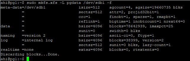
We verify the result:
ahi@pgl:~$ sudo blkid /dev/sdb1
/dev/sdb1: LABEL="pgdata" UUID="028afa2f-7bb3-4a40-92aa-91c1a33f18ae9" BLOCK_SIZE="512" TYPE="xfs" PARTUUID="bd54f285-092e-4b1b-ba5e-6877f054fa7"
We create the mount point:
sudo mkdir -p /pgdataPersistent mount via fstab:
We add the mount entry to /etc/fstab using the filesystem label rather than the device name. The device name (/dev/sdb) may change if disks are added or removed while the label remains stable:
echo 'LABEL=pgdata /pgdata xfs noatime,nodiratime 0 2' | sudo tee -a /etc/fstab
sudo systemctl daemon-reload
sudo mount /pgdata
We verify that the volume is mounted:
df -h /pgdata PostgreSQL installation
We install PostgreSQL 18 from the official PGDG repository, which provides the latest PostgreSQL versions for Ubuntu:
sudo apt install -y postgresql-common
sudo /usr/share/postgresql-common/pgdg/apt.postgresql.org.sh -y
sudo apt install -y postgresql-18
Cluster creation on /pgdata:
The Ubuntu packages create a default cluster under /var/lib/postgresql. This is not what we want. The data files and the WAL must both reside on the ZFS-backed volume, so that a single ZFS snapshot captures a consistent state of the database. If they were on different volumes, the snapshot would not be atomic.
We drop the default cluster and recreate it on /pgdata:
ahi@pgl:~$ sudo pg_dropcluster --stop 18 main
sudo install -d -o postgres -g postgres -m 700 /pgdata/18
sudo pg_createcluster -d /pgdata/18/main 18 main
sudo systemctl enable --now postgresql@18-main
Creating new PostgreSQL cluster 18/main ...
/usr/lib/postgresql/18/bin/initdb -D /pgdata/18/main --auth-local peer --auth-host scram-sha-256 --no-instructions
The files belonging to this database system will be owned by user "postgres".
This user must also own the server process.

The database cluster will be initialized with locale "en_US.UTF-8".
The default database encoding has accordingly been set to "UTF8".
The default text search configuration will be set to "english".

Data page checksums are enabled.

fixing permissions on existing directory /pgdata/18/main ... ok
creating subdirectories ... ok
selecting dynamic shared memory implementation ... posix
selecting default "max_connections" ... 100
selecting default "shared_buffers" ... 128MB
selecting default time zone ... Etc/UTC
creating configuration files ... ok
running bootstrap script ... ok
performing post-bootstrap initialization ... ok
syncing data to disk ... ok
             Ver Cluster Port Status Owner     Data directory  Log file
             18  main    5432 down   postgres  /pgdata/18/main /var/log/postgresql/postgresql-18-main.log
Created symlink /etc/systemd/system/multi-user.target.wants/postgresql@18-main.service → /usr/lib/systemd/system/postgresql@.service.
We verify that the cluster is online and located on the right volume:
ahi@pgl:~$ pg_lsclusters
Ver Cluster Port Status Owner     Data directory  Log file
18  main    5432 online <unknown> /pgdata/18/main /var/log/postgresql/postgresql-18-main.log
ahi@pgl:~$ sudo -u postgres psql -c "SHOW data_directory;"
 data_directory
-----------------
 /pgdata/18/main
(1 row)

ahi@pgl:~$ sudo -u postgres psql -c "SELECT version();"
                                                             version
-------------------------------------------------------------------------------------------------------------------------------
 PostgreSQL 18.4 (Ubuntu 18.4-1.pgdg24.04+1) on x86_64-pc-linux-gnu, compiled by gcc (Ubuntu 13.3.0-6ubuntu2~24.04.1) 13.3.0, 64-bit
(1 row)
We can also confirm that the WAL directory lives inside the data directory, and therefore on the zvol:
ls -ld /pgdata/18/main/pg_walWe need a database large enough to make traditional backup and restore operations time-consuming. In the SQL Server part of this series, we used the StackOverflow database (about 207 GB). For PostgreSQL, we use pgbench, the benchmarking tool shipped with PostgreSQL.
We create the database and initialize it with a scale factor of 10000. This produces a database of approximately 146 GB, with 1 billion rows in the pgbench_accounts table:
sudo -u postgres createdb bench
sudo -u postgres pgbench -i -s 10000 --partitions=8 bench
A few minutes later:

We can monitor the data growth during the initialization:
watch -n 30 'df -h /pgdata'
A few minutes later:

On the Proxmox side:
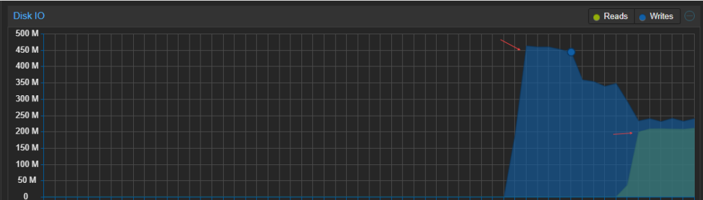
After some time, the process completes:
vacuuming...

creating primary keys...
done in 1559.55 s (drop tables 0.00 s, create tables 0.02 s, client-side generate 598.12 s, vacuum 675.53 s, primary keys 285.88 s).
ahi@pgl:~$
We check the database size:

We run a checkpoint before taking the snapshot. The recovery process starts replaying the WAL from the last checkpoint. By running it right before the snapshot, almost nothing needs to be replayed when the database starts after a restore:
sudo -u postgres psql -c "CHECKPOINT;"
Comparison with SQL Server:
On the SQL Server side, we had to run SUSPEND_FOR_SNAPSHOT_BACKUP and BACKUP WITH METADATA_ONLY. On the PostgreSQL side, none of that is needed.
The data files and the WAL are on the same zvol. An atomic ZFS snapshot therefore captures a state equivalent to a power loss, and PostgreSQL is designed to recover cleanly from that state through crash recovery: the WAL is replayed from the last checkpoint. This is documented and officially supported.
The snapshot is the backup. There is no .bkm file, no metadata backup.
SQL ServerPostgreSQLBefore the snapshotALTER DATABASE…SET SUSPEND_FOR_SNAPSHOT_BACKUP = ONCHECKPOINT (optional)Backup recordBACKUP WITH METADATA_ONLYNoneDuring the restoreRESTORE WITH METADATA_ONLYAutomatic crash recovery (WAL replay)Evidence in the logs“I/O is frozen” in the ERRORLOG“redo starts/redo done” in the PostgreSQL log Snapshot process flowOn the Proxmox side, we create the snapshot and protect it with a hold:
SNAP="sqlpool/pve/vm-307-disk-0@pg_bench_$(date +%Y%m%dT%H%M%S)"
zfs snapshot "$SNAP"
zfs hold sqlsnap "$SNAP"
echo "$SNAP"
The hold protects the snapshot from an accidental destruction, as we did in part 2 of this series. We note the exact snapshot name, it will be needed for the restore.
The database stays online during the whole operation. No I/O freeze is required.
We list the snapshots:
zfs list -t snapshot -r sqlpool/pve/vm-307-disk-0
We drop the database then we restore the snapshot:
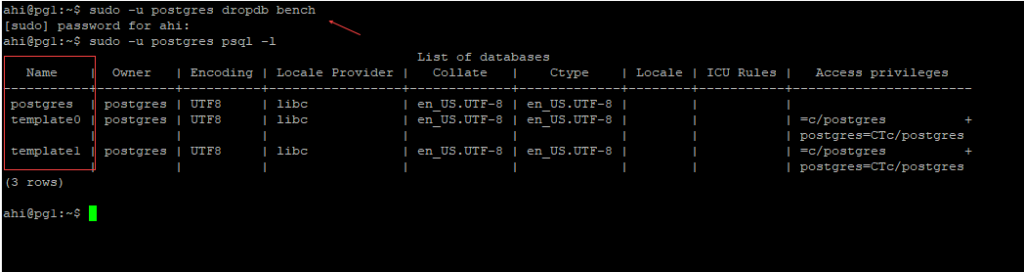
We run the snapshot restore procedure. On the VM, we stop the cluster and unmount the volume:
sudo systemctl stop postgresql@18-main
sudo umount /pgdata
On the Proxmox side, we want to restore our snapshot. We can list the available snapshots:
zfs list -t snapshot -r sqlpool/pve/vm-307-disk-0
We roll back the snapshot:
zfs rollback -r sqlpool/pve/vm-307-disk-0@pg_bench_20260803T165409On the VM, we mount the volume and start the service:
sudo mount /pgdata
sudo systemctl start postgresql@18-main
We check a few elements in the logs:
sudo tail -30 /var/log/postgresql/postgresql-18-main.logThe service shutdown, then the restart:
UTC [232108] LOG:  database system is shut down
UTC [233968] LOG:  starting PostgreSQL 18.4 (Ubuntu 18.4-1.pgdg24.04+1) on x86_64-pc-linux-gnu, compiled by gcc (Ubuntu 13.3.0-6ubuntu2~24.04.1) 13.3.0, 64-bit
UTC [233968] LOG:  listening on IPv4 address "0.0.0.0", port 5432
UTC [233968] LOG:  listening on IPv6 address "::", port 5432
UTC [233968] LOG:  listening on Unix socket "/var/run/postgresql/.s.PGSQL.5432"
PostgreSQL detects that the database was not shut down properly and replays the WAL. This is the same crash recovery mechanism as in SQL Server. Finally, the database starts.
UTC [233974] LOG:  database system was not properly shut down; automatic recovery in progress
UTC [233974] LOG:  redo starts at 20/2CB76278
UTC [233974] LOG:  invalid record length at 20/2CB76380: expected at least 24, got 0
UTC [233974] LOG:  redo done at 20/2CB76348 system usage: CPU: user: 0.00 s, system: 0.00 s, elapsed: 0.00 s
UTC [233974] LOG:  checkpoint starting: end-of-recovery immediate wait
UTC [233972] LOG:  checkpoint complete: wrote 0 buffers (0.0%), wrote 3 SLRU buffers; 0 WAL file(s) added, 0 removed, 0 recycled; write=0.002 s, sync=0.009 s, total=0.030 s; sync files=0, longest=0.000 s, average=0.005 s; distance=0 kB, estimate=0 kB; lsn=20/2CB76380, redo lsn=20/2CB76380
UTC [233968] LOG:  database system is ready to accept connections
We then verify that the database is available again:
sudo -u postgres psql -d bench -c "SELECT pg_size_pretty(pg_database_size('bench'));" Consistency proof under load
The previous test was done on a quiesced database: we ran a CHECKPOINT right before the snapshot, and nothing was writing. The real question is: what happens if the snapshot is taken while the database is being written to?
This is where PostgreSQL differs the most from SQL Server. There is no SUSPEND_FOR_SNAPSHOT_BACKUP. We take the snapshot in the middle of the write activity and we let the WAL replay do the work.
We start the load. The built-in pgbench script runs a TPC-B-like transaction: three UPDATE statements on the accounts, tellers and branches tables and one INSERT into the history table:
sudo -u postgres pgbench -c 8 -j 4 -T 300 bench &
While the load is running, we take a snapshot on the Proxmox side:
zfs snapshot sqlpool/pve/vm-307-disk-0@pg_bench_$(date +%Y%m%dT%H%M%S)

zfs hold sqlsnap sqlpool/pve/vm-307-disk-0@pg_bench_20260803T224551
No CHECKPOINT this time, no freeze. The database is actively writing while the snapshot is taken.
The state after some time under load:
We stop the service:
sudo systemctl stop postgresql@18-main
sudo umount /pgdata
We restore the snapshot:
zfs rollback -r sqlpool/pve/vm-307-disk-0@pg_bench_20260803T224551 
We mount the volume, start the service and check the logs:
sudo mount /pgdata
sudo systemctl start postgresql@18-main
This time the log shows a real recovery:
2026-08-03 20:49:03.244 UTC [234405] LOG:  database system is shut down
2026-08-03 20:50:34.333 UTC [234620] LOG:  starting PostgreSQL 18.4 (Ubuntu 18.4-1.pgdg24.04+1) on x86_64-pc-linux-gnu, compiled by gcc (Ubuntu 13.3.0-6ubuntu2~24.04.1) 13.3.0, 64-bit
2026-08-03 20:50:34.333 UTC [234620] LOG:  listening on IPv4 address "0.0.0.0", port 5432
2026-08-03 20:50:34.333 UTC [234620] LOG:  listening on IPv6 address "::", port 5432
2026-08-03 20:50:34.335 UTC [234620] LOG:  listening on Unix socket "/var/run/postgresql/.s.PGSQL.5432"
2026-08-03 20:50:34.343 UTC [234626] LOG:  database system was interrupted; last known up at 2026-08-03 20:44:36 UTC
2026-08-03 20:50:34.381 UTC [234626] LOG:  database system was not properly shut down; automatic recovery in progress
2026-08-03 20:50:34.384 UTC [234626] LOG:  redo starts at 20/7A3618B0
2026-08-03 20:50:38.024 UTC [234626] LOG:  invalid record length at 20/8BC0A4F8: expected at least 24, got 0
2026-08-03 20:50:38.024 UTC [234626] LOG:  redo done at 20/8BC0A4D0 system usage: CPU: user: 0.71 s, system: 0.63 s, elapsed: 3.63 s
2026-08-03 20:50:38.028 UTC [234624] LOG:  checkpoint starting: end-of-recovery immediate wait
2026-08-03 20:50:53.936 UTC [234624] LOG:  checkpoint complete: wrote 105355 buffers (53.6%), wrote 5 SLRU buffers; 0 WAL file(s) added, 17 removed, 0 recycled; write=3.648 s, sync=12.232 s, total=15.911 s; sync files=189, longest=12.223 s, average=0.065 s; distance=287395 kB, estimate=287395 kB; lsn=20/8BC0A4F8, redo lsn=20/8BC0A4F8
2026-08-03 20:50:53.948 UTC [234620] LOG:  database system is ready to accept connections
Three differences compared to the first test:
- The “last known up at” timestamp (20:44:36) does not match a checkpoint we ran manually. It matches the last automatic checkpoint triggered during the load.
- The redo is not instantaneous anymore: 3.63 seconds, replaying about 280 MB of WAL (from LSN 20/7A3618B0 to 20/8BC0A4D0). All the write activity between the last checkpoint and the snapshot had to be replayed. The transactions committed before the snapshot are recovered, the ones that were in flight are rolled back.
- The end-of-recovery checkpoint then writes everything the redo rebuilt in memory: 105355 buffers, 53.6% of the buffer pool. The database is ready to accept connections about 19 seconds after the service start.
The crash recovery completed correctly and the database has been restored. We verify the TPC-B invariant. Each pgbench transaction applies the same delta to the accounts, tellers and branches tables in a single transaction. On a consistent database, the three sums must be equal:
 Major drawbacks
- The snapshot covers the whole zvol. All the databases of the cluster are captured and restored together. There is no per-database restore, unlike the METADATA_ONLY approach on SQL Server which targets a single database.
- There is no backup history. SQL Server records the metadata backup in msdb. Here, the only trace is the snapshot itself on the ZFS side.
- Point-in-time recovery is not covered. The snapshot alone brings the database back to the moment it was taken. For PITR, WAL archiving would still be required on top of it.
- The snapshot backup and restore model of the SQL Server series applies to PostgreSQL (no I/O freeze, no metadata backup).
- One important rule: data files and WAL must reside on the same zvol so the snapshot is atomic.
- A 146 GB database was restored in a few seconds and in less than 20 seconds under active load, WAL replay included.
Thank you. Amine Haloui
L’article PostgreSQL Snapshot Backup and Restore with Proxmox ZFS (4/4) est apparu en premier sur dbi Blog.
Customer experience – Certificat SSL on an SQL Server Reporting Services
Recently, I had to renew an SSL certificate on an SQL Server Reporting Services (SSRS) server. The task seemed straightforward: replacing an expired certificate with a new one containing the same configuration. However, once the change had been made, HTTPS wasn’t working anywhere — neither via the usual DNS names nor even when accessing the server directly. Only HTTP remained accessible.
Here is a step-by-step guide to how the problem was solved.
SymptomAfter the certificate was renewed:
- HTTP was working normally, both remotely and locally.
- HTTPS was not working.
- There were no certificate warnings or TLS errors: the issue manifested as an application error (404).
A 404 error is an application error, not an encryption error. It means that the TLS connection was established correctly (the certificate was presented and accepted), but that the server could not find any resource matching the request.
 Step 1: Check the installed certificate
The first thing to check in any case is the certificate. Go to the server certificates and select the proprieties of the right certificate. You must ensure that it does indeed contain the correct SANs (Subject Alternative Names).
A point that is often overlooked: the CN (Common Name) of a certificate is no longer considered 100 per cent reliable. If you wish to connect via HTTPS using a specific name . That name must be included in the certificate’s SAN field, and not just in the CN.
Step 2: Check the SSRS configurationThe next step is to check the configuration of SSRS itself:
- Check that the certificate has been correctly associated with the service in Reporting Services Configuration Manager (Web Service URL and Web Portal URL).
- Check that the certificate is recognised for both IPv4 and IPv6.
- Ensure that the binding is consistent on both the SSRS service side and the server side (Windows / HTTP.sys).
This final check can be carried out via the command line using:
netsh http show sslcertThis command lists the mappings between IP addresses/ports and certificates (identified by their hash). In my case, the binding was set up using wildcards (0.0.0.0:443 and [::]:443) with a single certificate for all incoming HTTPS requests on port 443.
 Step 4: URL Reservations
It was whilst looking into reserved URLs that the problem came to light. The following command lists the URLs reserved with HTTP.sys, the Windows component that manages HTTP/HTTPS listening at the system level:
netsh http show urlaclThe result revealed the source of the problem: the entries did indeed exist, but only for the server name, with an explicit host header. However, as the server name was not present in the certificate’s SAN. This is why the HTTPS connection was not working either:
 Reserve the right URLs
The fix involves recreating the reservations assigned to each DNS so that the host header is accepted. Here, we add the URL by specifying the service account. It is important to add the SDDL (Security Descriptor Definition Language) . This is used to grant service accounts (like ReportServer) the permissions required to reserve specific URLs for web traffic. For SSRS 2017 and later, the AccountSid value is S-1-5-80-4050220999-2730734961-1537482082-519850261-379003301 and the AccountName value is NT SERVICE\SQLServerReportingServices. For Power BI Report Server, the AccountSid value is S-1-5-80-1730998386-2757299892-37364343-1607169425-3512908663 and the AccountName value is NT SERVICE\PowerBIReportServer. Here, we use the specifications for SSRS
cmd
netsh http add urlacl  url=https://"dns.name":443/Reports
user="NT Service\ReportServerSQLServerReportingServices" sddl=D:(A;;GX;;;S-1-5-80-4050220999-2730734961-1537482082-519850261-379003301)

netsh http add urlacl  url=https://"dns.name":443/ReportServer
user="NT Service\SQLServerReportingServices" sddl=D:(A;;GX;;;S-1-5-80-4050220999-2730734961-1537482082-519850261-379003301)
Once the previous steps had been completed without any issues being detected, the certificate contained the correct SANs, the SSRS configuration appeared to be consistent, and the DNS records were correctly pointing to the correct IP address. we had to dig deeper into the service’s configuration file itself:
C:\Program Files\Microsoft Power BI Report Server\PBIRS\ReportServer\rsreportserver.config
Contrary to what one might think, URL reservations at the HTTP.sys level (netsh http show urlacl) are not sufficient on their own: the SSRS/PBIRS service also maintains its own list of authorised names directly within this configuration file. Additions must be made after this tag : one entry for the web service (/ReportServer/) and another for the web portal (/Reports/). If a DNS entry is not explicitly declared in both of these locations, the service may refuse to recognise it as a valid name, even though HTTP.sys would be prepared to allow the request through.
The fix therefore involves manually editing the rsreportserver.config file and adding each relevant DNS to both instances of the tag, whilst strictly adhering to the syntax already in place for the existing entries.
Once changes have been made, the service must be restarted for the changes to take effect.
 In summary
So here are a few key points to bear in mind:
- A 404 error over HTTPS following a certificate change is not necessarily related to the certificate itself. If the TLS connection is established without any warnings, the problem is likely to lie in application routing (URL reservations), not in the trust chain.
netsh http show urlaclandnetsh http show sslcertare the two key commands for distinguishing between a certificate binding issue and a URL reservation issue.- An explicit host header (name:443) restricts access to that name only
- The service account is just as important as the URL itself. A technically correct reservation that is associated with the wrong account will prevent the service from creating its own endpoint, resulting in an E_ACCESSDENIED error on start-up.
Some Sources:
About reservations URL :Configure Reporting Services to use a Subject Alternative Name (SAN) – SQL Server Reporting Services (SSRS) | Microsoft Learn
About Common name on certificat : Chrome 58: Common Name in SSL Certificates Finally Dies | Dataprise
L’article Customer experience – Certificat SSL on an SQL Server Reporting Services est apparu en premier sur dbi Blog.
When an idle transaction starves the worker pool (THREADPOOL)
A production instance, mid-afternoon, nothing unusual on any dashboard. An engineer opens a transaction to patch a single row while investigating a data issue:
BEGIN TRANSACTION;
UPDATE dbo.Orders SET Status = 'Reviewed' WHERE OrderId = 482193;
No COMMIT. No ROLLBACK. The tab gets buried under three others, the investigation moves on, and the lock is still held an hour later.
Every query, every batch, every login needs a worker thread to execute on. That pool is not infinite, it is sized by max worker threads, either left on its computed default or pinned to a fixed number.
SELECT name, value_in_use FROM sys.configurations WHERE name = 'max worker threads';

name                                value_in_use
----------------------------------- -------------------------------------------------------------------------------------------------------------------------
max worker threads                  128
SQL Server schedules work cooperatively, not preemptively. Each worker is handed a quantum (4 milliseconds) to run before it is expected to voluntarily yield the scheduler to the next runnable task. This is the mechanism behind SOS_SCHEDULER_YIELD: a worker that still has work to do, but whose quantum has expired, stepping aside so someone else gets a turn.
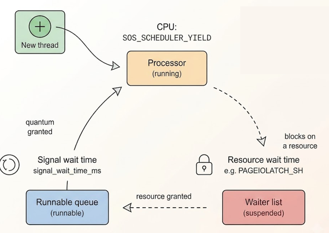
None of this applies to the open transaction from earlier. A session that has issued no command has no task and holds no worker. Its status in sys.dm_exec_sessions is sleeping, not running, not suspended.
SELECT
    s.session_id,
    s.status AS session_status,
    ct.text
FROM sys.dm_exec_sessions s
LEFT JOIN sys.dm_exec_requests r ON s.session_id = r.session_id
LEFT JOIN sys.dm_exec_connections c ON s.session_id = c.session_id
OUTER APPLY sys.dm_exec_sql_text(c.most_recent_sql_handle) ct
WHERE s.session_id = 54;

session_id session_status                 text
---------- ------------------------------ --------------------------------------------------------------------------------------------------------------------
54         sleeping                       UPDATE dbo.Orders SET Status = 'Reviewed' WHERE OrderId = 482193;
It is not waiting for a quantum, because it is not competing for one. The lock it holds costs the engine nothing in scheduling terms; it is bookkeeping in the lock manager, entirely separate from the worker pool.
Two hundred sessions walk into a lockLet’s say that the application wants to confirm that the orders has been reviewed now it’s in the processed state.
BEGIN TRANSACTION;
UPDATE dbo.Orders SET Status = 'Processed' WHERE OrderId = 482193;
Seeing that the query didn’t complete to update the item, it will keep sending this transaction again and again, sending it 200 times let’s say.
Unlike the sleeping session above, each of these has issued a command. Each one is granted a worker to execute it, immediately hits the lock, and transitions to suspended, waiting on LCK_M_X.
wait_type                   waiting_tasks_count       wait_time_ms
THREADPOOL                      521                      2881770
SOS_SCHEDULER_YIELD             710                      41
 session_id     status        wait_type        wait_time   blocking_session_id
    68         suspended       LCK_M_X          29873             54
   ...
   206         suspended       LCK_M_X          29478             68
   207         suspended       LCK_M_X          29478             68
scheduler_id runnable_tasks_count work_queue_count active_workers_count
       0              0               19                 43
       1              0               5                  45
       2              0               10                 45
       3              0               2                  44
active_workers    max_workers_count
         205                    128
Note: max_workers_count only counts the user-facing pool; internal system threads, including the DAC’s own reserved worker used to capture this very output, sit outside that ceiling.
The worker is not released while the task waits. It stays attached to the suspended task for the entire duration of the block, doing nothing, simply reserved, waiting for the resource (the order line to update) to be available for updates.
The remainder cannot even be granted a worker to start waiting. They queue behind everyone else, and eventually give up entirely:
Login timeout expired
Login/Query timeout: 15/0 seconds
By this point the server has simply stopped accepting new connections.
When the fire exit is also on fireReleasing the original lock should be the easy part: switch back to the session from the very first transaction, issue a ROLLBACK, and watch everything clear. Except that session, which has been sitting sleeping and worker-free this whole time, now has to issue a command of its own. And issuing a command means asking the pool for a worker (the same exhausted pool every other session is already queued for). The session responsible for the deadlock has no priority for fixing it. It gets in line like everyone else, behind two hundred sessions it created the conditions for.
This is where the Dedicated Admin Connection comes in the game. It runs on its own scheduler, with a worker reserved outside the regular pool, built specifically for an instance too exhausted to serve itself.
sqlcmd -A -S"." -E
SELECT blocking_session_id
FROM sys.dm_exec_requests
WHERE blocking_session_id <> 0;

KILL 54;
Note: the “.” here resolves to the local default instance but unlike an ordinary local connection (which typically uses Shared Memory), the DAC always connects over its own dedicated TCP listener on the loopback adapter, regardless of protocol settings on the port 1434 or a dynamic one (full documentation here).
The KILL forces the rollback from outside the exhausted pool entirely. Workers free up in cascade, and the two hundred suspended sessions complete their updates and release their own.
In this example, we set the parameter max worker threads to 128 to easily saturate the worker threads. However, the default value for max worker threads is 0, which lets SQL Server compute the number of worker threads automatically at startup based on the number of logical CPUs and the platform architecture. Microsoft best practice can be found here and shows the following table:
And the key take-away from this experiment:
- Sleeping costs nothing, suspended costs a worker. The distinction between an idle transaction and a blocked one is the entire mechanism behind this incident: both hold a lock, only one of them holds a thread.
- The scheduler’s quantum explains CPU pressure, not threadpool exhaustion. Yielding after 4ms is about sharing a CPU among runnable workers; it has nothing to do with how many workers exist in the first place.
- The session that caused the block is not exempt from the consequences of the block. It has to compete for a worker like anything else, the moment it tries to clean up after itself.
- Never let a statement end without a
COMMITor aROLLBACK.
L’article When an idle transaction starves the worker pool (THREADPOOL) est apparu en premier sur dbi Blog.
Why search is the most underrated ECM feature
When organizations evaluate an Enterprise Content Management (ECM) solution, the conversation usually revolves around Artificial Intelligence, workflow automation, and integrations.
Yet the feature employees use more than any other is rarely the one showcased in demonstrations or marketing brochures: search.

The reality is simple. Most users don’t spend their days creating workflows or configuring metadata. They spend it looking for information.
Every unsuccessful search comes at a cost!
Search happens more often than you thinkThink about your workday.
How many documents do you create?
Maybe a few.
How many do you approve?
Perhaps a few more.
Now, ask yourself a different question: How many times do you search for information?
Procedures, invoices, contracts, customer communications…
For most employees, searching is the most common interaction with an ECM system by far.
This means that even minor improvements to the search function can significantly impact productivity.
Finding a document is only half the problemMany ECM vendors claim they can find any document in seconds.
That’s great, but it’s often not enough.
Imagine a customer calls about an invoice. You know the supplier, but not the invoice number.
A good ECM lets you find the document in seconds by searching the supplier, project, purchase order, or even the contract linked to it.
A poor search experience forces you to browse folders, ask colleagues, or search through emails.
An effective search is about relevance, not just speed.
Search starts long before someone types a keywordMany organizations try to improve their search function by tweaking the search engine.
In reality, a good search starts much earlier.
It begins with:
- meaningful metadata
- consistent naming conventions
- well-designed object relationships
- document classifications
- quality-controlled information
Poor information management cannot be fixed with search alone.
Even the most advanced search engine will struggle to deliver useful results if the metadata is inconsistent or incomplete.
Search should reduce decisionsA good search experience should minimize the amount of thought required of users.
Instead of asking:
“What was the exact document name?”
Users should be able to search naturally:
- customer name
- supplier
- project
- Invoice number
- Contract type
- Date
- Keywords
The system should handle the complexities.
Users shouldn’t need to understand how the information is stored.
What about AI?Generative AI doesn’t replace search, it changes users’ expectations of search.
Now users want to be able to ask questions like:
“Show me all contracts that expire next quarter.”
Or:
“Find the latest approved procedure for handling customer complaints.”
Behind these simple questions lies something much less glamorous: reliable metadata.
Without it, AI cannot consistently provide trustworthy answers.
In many ways, AI has made search even more important.
Search is a user experience featureWhen discussing user adoption, project teams often focus on training.
Training certainly matters.
However, the user experience during searches is also important.
If employees consistently find what they need in seconds, their confidence in the system grows.
However, if they repeatedly fail to find information, they’ll quickly return to shared drives, email folders, or ask colleagues for help.
The quality of the search function shapes the perception of the entire enterprise content management (ECM) solution.
Search is a business capabilityA good search is about more than just saving a few minutes.
- It enables better decision-making.
- It prevents duplicate work.
- It improves compliance.
- It accelerates customer service.
- It helps preserve organizational knowledge.
The value of an ECM system isn’t measured by how many documents it stores.
Rather, it’s measured by how effectively those documents can be found and used.
Final wordsSearch rarely appears as the headline feature in product demonstrations because every ECM platform offers some form of search.
The real difference isn’t whether a system can search, it’s how effectively users can find the right information when they need it.
A successful ECM implementation isn’t one where information is simply stored.
Rather, it’s one where information is found effortlessly, trusted confidently, and reused effectively.
After all, a document that can’t be found might as well not exist.
L’article Why search is the most underrated ECM feature est apparu en premier sur dbi Blog.
Zabbix Agent 2 service terminated unexpectedly on Windows server
The Zabbix Agent 2 service on a Windows server was repeatedly becoming unresponsive and eventually crashing. The issue caused intermittent monitoring interruptions and required further investigation through Event Viewer messages and Zabbix Agent 2 logs to better understand why the service was no longer responding properly.
While monitoring a Windows server with Zabbix Agent 2, we encountered repeated crashes of the agent service accompanied by the following Event Viewer message:
A timeout (30000 milliseconds) was reached while waiting for a transaction response from the Zabbix Agent 2 service.
A few moments later, Windows reported:
The Zabbix Agent 2 service terminated unexpectedly.
The first assumption was that a plugin or item was taking too long to execute, causing the agent to become unresponsive. A natural idea was therefore to increase the timeout value. Here the official documentation for the PluginTimout.
Inside the Zabbix Agent 2 configuration, we identified the following parameter:
### Option:PluginTimeout
# Timeout for connections with external plugins.
## Mandatory: no
# Range: 1-30
# Default: <Global timeout>
# PluginTimeout=
However, this parameter only supports values between 1 and 30 seconds.
This raised an important question:
If a timeout already exists, why does the entire agent still become blocked and eventually crash?
Understanding the ProblemZabbix Agent 2 uses a plugin-based architecture written in Go.
Unlike isolated external processes, many plugins run inside the same agent process.
This means that if a plugin becomes blocked:
- worker threads remain occupied
- new requests start queuing
- the agent gradually stops responding
- Windows eventually considers the service frozen
The 30-second timeout seen in Event Viewer is actually the Windows Service Control Manager (SCM) timeout, not a protection mechanism for the plugin itself.
In other words:
- the plugin blocks first
- the agent becomes unresponsive
- Windows waits 30 seconds
- Windows kills the service
The Zabbix Agent 2 logs quickly pointed toward the real culprit.
[WindowsPerfMon] failed to get performance counters data:'cannot collect value No data to return.'
This indicated that the agent was struggling to collect Windows Performance Counters.
The most important recurring message was:
[WindowsPerfInstance] Cannot refresh object cache:Unable to connect to the specified computer or the computer is offline.
This error appeared continuously for several days.
The key observation here is that the agent was running locally, so the message below should never normally appear:
Unable to connect to the specified computer
This strongly suggested:
- an invalid or corrupted performance counter
- a problematic PerfMon object
- or a failing wildcard instance (
Process(*),LogicalDisk(*), etc.)
Later in the logs, additional symptoms appeared:
failed to accept an incoming connection:accept tcp [::]:10050:acceptex: The I/O operation has been aborted because of either a thread exit or an application request.
At this stage, the agent was no longer able to accept incoming connections because its internal workers were saturated or blocked.
This confirmed that the issue was not a traditional crash, but rather a thread starvation / blocking situation.
Why the Existing 30s Timeout Was Not EnoughAn important misunderstanding was clarified during the investigation.
The default timeout value of 30 seconds does not immediately protect the agent.
Instead:
- the plugin may block for the full 30 seconds
- multiple blocked requests accumulate
- worker threads remain occupied
- the agent becomes globally unresponsive
By the time Windows notices the issue, the agent is already effectively frozen.
The Solution: Reduce PluginTimeoutInstead of increasing the timeout, the correct approach was to reduce it significantly.
The following configuration was applied:
PluginTimeout=15
This acts as a protection mechanism inside the agent itself.
With this configuration:
- problematic plugin executions are aborted quickly
- blocked threads are released faster
- the agent remains responsive
- only the affected items temporarily fail
The issue was not caused by the timeout itself.
The real root cause was a problematic WindowsPerfInstance plugin execution blocking the Zabbix Agent 2 internal workers.
Reducing the plugin timeout from 30 seconds to 15 seconds prevented the entire agent from becoming unresponsive while still allowing the monitoring system to recover automatically when the plugin started responding again.
This is a good example of why increasing timeouts is not always the right solution. Sometimes, shorter timeouts are actually what keeps a monitoring agent stable.
You can find other blogs regarding Zabbix or database administration or other topics at this link: dbi blogs
L’article Zabbix Agent 2 service terminated unexpectedly on Windows server est apparu en premier sur dbi Blog.
Oracle GenAI – Ask EM – Deploy Oracle Enterprise Manager 24ai from Marketplace
I have been looking to study and test what Oracle GenAI Ask EM assistant, also called now Oracle AI database assistant, can offer. This generative AI assistant is directly integrated into Oracle Enterprise Manager 24ai. Before being able to look into Ask EM, I first had to install an Oracle EM platform. I had the choice between doing all the installation myself manually or installing it from Oracle Marketplace. Knowing my current need, I decided to install it from the Oracle Marketplace. I would like to share in this first Ask EM series blogs this installation.
Pros and Cons for a Marketplace installationFor my current purpose of getting a lab in order to test GenAI Ask EM feature, the advantages of doing an installation from the marketplace are the following:
- Faster and less work to get a working environment ready for Ask Em testing
- Less possible errors and problems
- Oracle prope a full preconfigured image with OS and EM
- Minimalize deployement time
- More time to focus on Ask EM testing
The disadvantage would be to have:
- Less flexibility
But I really do not need any customized installation.
The manual installation complexity would mainly be to install and configure manually:
- Oracle VM with OS (Oracle Linux)
- EM repository database
- EM weblogic
- EM software installation and patching
- OMS
- …
Please note following:
- I will be installing a simple deployment sizing lab.
- Enterprise Manager Instance Shape, VM.Standard2.4, will then be suffisient.
- I will use existing VCN and subnet
- I will make a single node installation with Enterprise Manager and database installed in a private subnet. This will have the benefit not to expose the Instance on the public network. I will then need a bastion VM which will be part of the installation
But what would be the cost? The cost will come mainly from the cost of the components:
- Compute instance will be charged based on the shape, OCPU and memory. It is in general the biggest cost
- Block Volume which is charged per provisioned GB
- Networking. VCN, subnets and security lists are free of charge, and are anyhow already existing.
- Single instance repository database does not require any license
- Use EM features only covered by your existing oracle licenses. Pack such as the Diagnostics Pack, Tuning Pack, Lifecycle Management Pack, etc., require the appropriate licenses.
The EM stack from the Marketplace is with BYOL (Bring Your Own License). In any case, I will strongly recommend to check your license and evaluate the cost on your side before doing any installation, moreover if it is for a production installation. My case is just a lab testing case.
Oracle Enterprise Manager 24ai installationI will first sign in to OCI and go to Marketplace. From there I will search and click on Oracle Enterprise Manager, see below pictures.
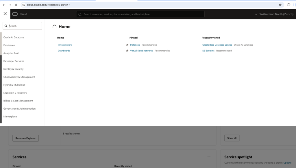
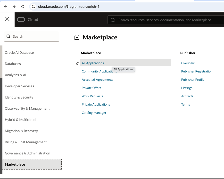
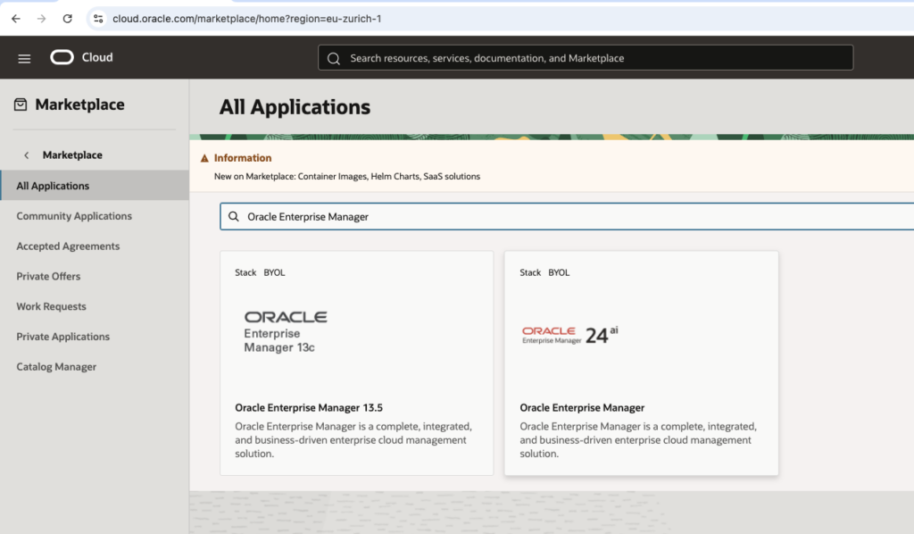
Once you have selected the Oracle Enterprise Manager 24ai stack, review the information to ensure it is accurate and click on Launch State.
Following 3 pictures will show the details.
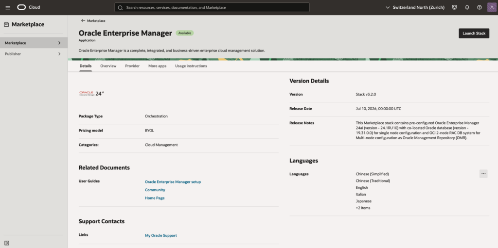
Configure Compartment, accept the terms and conditions and launch the stack, see:
Provide a name and a desciption, and click next, see:
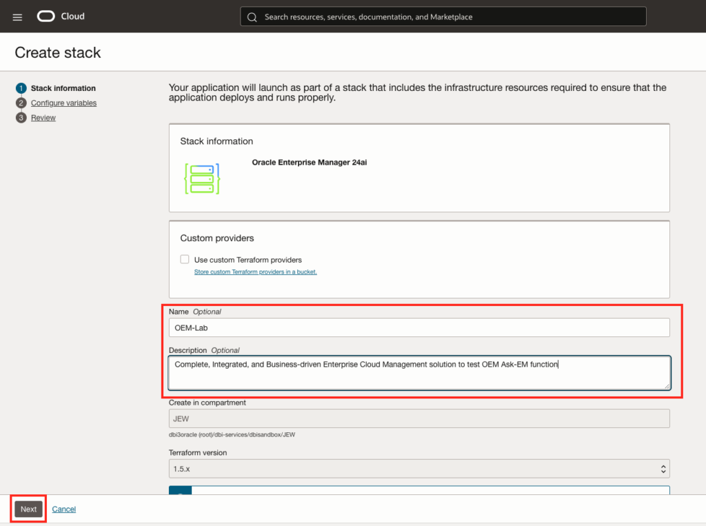
Configure the installation and sizing details:
- Choose simple as deployment size. One node is suffisient for our lab and test
- Click on advanced deployment to reuse existing infracsture (VCN and subnets)
See following picture:
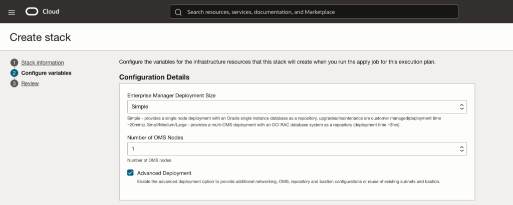
Provide existing VCN Name:
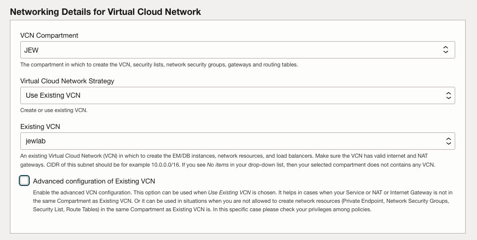
Provide networking details making sure to chose existing private subnet:
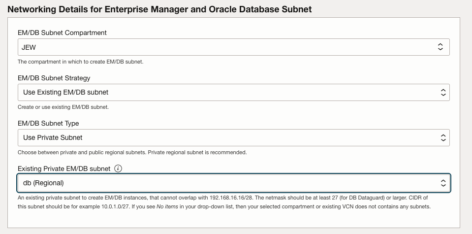
Configure Oracle Management providing Server details.
First we will provide an hostname prefix, choose Operating System version and provide Enterprise Manager password:
We will provide agent registration password and weblogic admin and node manager password, before chosing Enterprise Manager Instance shape and boot volume size. As discussed in the pre-requirement, a VM.Standard2.4 is enough for my need.
And finally also provide the public key to be able to access the VM later on with SSH.
I will also have to provide all the details concerning the repository database, that’s to say database sys and dnsnmp user password. I will keep the database in archive log mode.
As I choose to install Enterprise Manager in the private subnet, I will need a bastion. I could decide to use an existing one where the installation will make needed changes or create a new one specific for EM. I decided to create a new one, but using existing subnet, see following information that needs to be provided, before clicking next button:
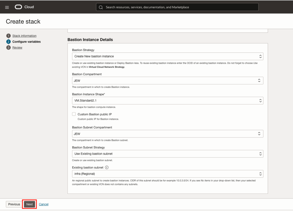
Review the whole configuration:
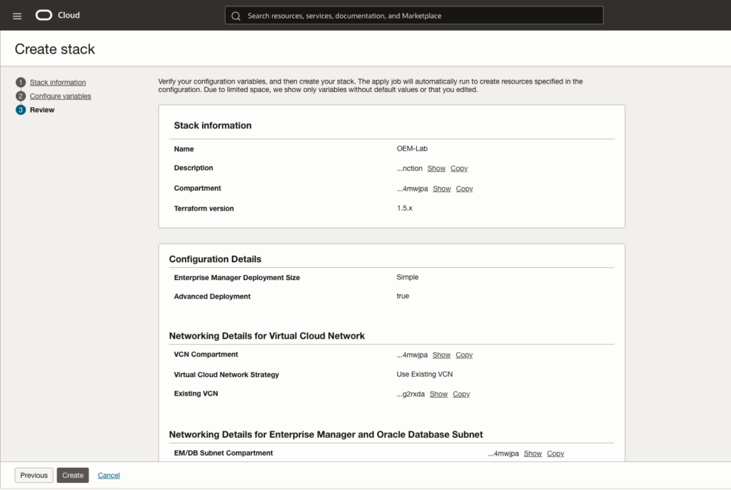
Select run apply and click the create button.
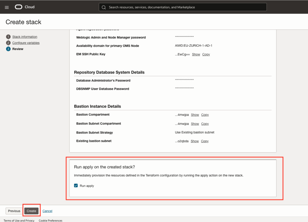
And the we can see the job stack execution. The status will first go to Accepted status and then In progress status, see next pictures:
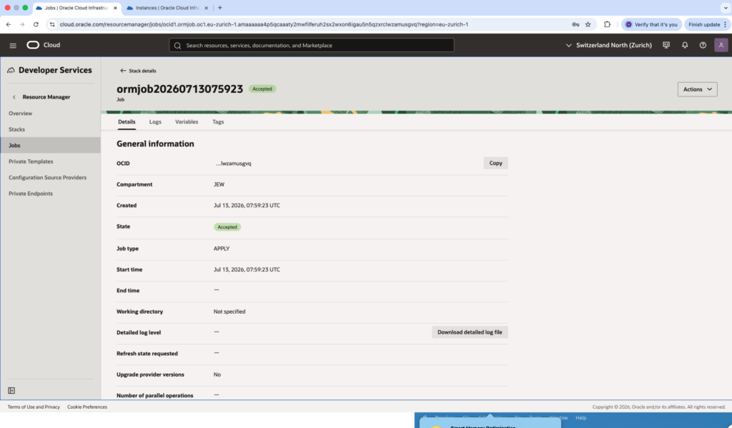
 Checks…
Once completed, we can check the job stack status, the created VM compute instance (OMS server, bastion) and EM access.
Job stackAs we can see in the next picture, the job status is now Succeeded.
In Resource Manager, under Stacks menu, we can see our OEM-Lab stack that is active. All components information will be provided.
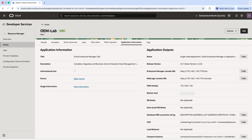 Compute VM instances
We can check in our compartment the running EM-OMS VM compute instance and EM-OMS-bastion.
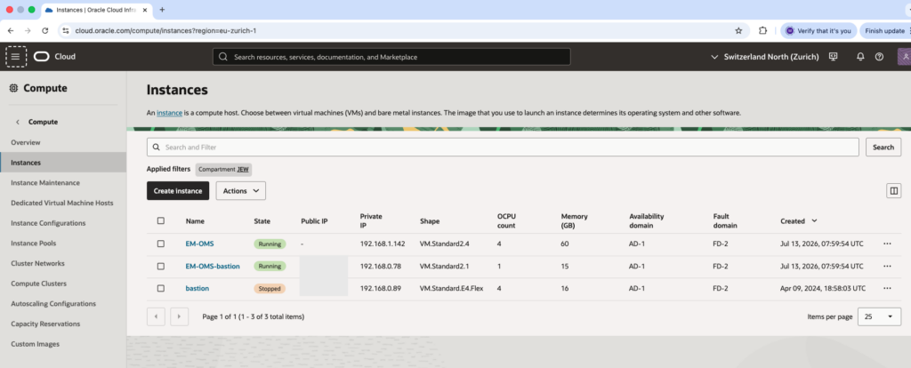 EM Web access
Let’s first check and confirm that I can join the OMS Bastion from my MAC.
maw@DBI-LT-MAW2 ~ % ssh -i /Users/maw/Documents/Current-Dokument/Dokument/pem_ssh_key/yak_beta_workshop/srv/sshkey opc@152.67.XX.XXX
The authenticity of host '152.67.XX.XXX (152.67.XX.XXX)' can't be established.
ED25519 key fingerprint is: SHA256:CVPCXt9EwZ153fUVnZf3AGADYNVqT9fJGaU70TKbX+I
This key is not known by any other names.
Are you sure you want to continue connecting (yes/no/[fingerprint])? yes
Warning: Permanently added '152.67.XX.XXX' (ED25519) to the list of known hosts.
** WARNING: connection is not using a post-quantum key exchange algorithm.
** This session may be vulnerable to "store now, decrypt later" attacks.
** The server may need to be upgraded. See https://openssh.com/pq.html
Last login: Mon Jul 13 08:25:33 2026 from 140.238.169.22
[opc@em-oms-bastion ~]$
AS I choose an installation on private network, I do not have access to EM through a web browser from my MAC. I first need to configure a ssh tunnel.
maw@DBI-LT-MAW2 ~ % ssh -i /Users/maw/Documents/Current-Dokument/Dokument/pem_ssh_key/yak_beta_workshop/srv/sshkey -L 7799:192.168.1.142:7799 opc@152.67.XX.XXX
** WARNING: connection is not using a post-quantum key exchange algorithm.
** This session may be vulnerable to "store now, decrypt later" attacks.
** The server may need to be upgraded. See https://openssh.com/pq.html
Last login: Mon Jul 13 11:02:53 2026 from 146.4.101.46
[opc@em-oms-bastion ~]$
Check from OMS bastion that EM console is reachable.
[opc@em-oms-bastion ~]$ curl -k https://192.168.1.142:7799/em 302 Moved TemporarilyThis document you requested has moved temporarily.
It's now at https://192.168.1.142:7799/em/login.jsp.
[opc@em-oms-bastion ~]$
Check that the connection is possible on EM from my MAC directly after I have created the SSH tunnel:
maw@DBI-LT-MAW2 ~ % curl -k https://localhost:7799/em 302 Moved TemporarilyThis document you requested has moved temporarily.
It's now at https://localhost:7799/em/login.jsp.
maw@DBI-LT-MAW2 ~ %
All is good, I can not test from my MAC using a web browser.
Let’s go in the summary page.
 To wrap up…
The easiest way for me to have got a EM lab installation to look into GenAI Ask EM was to install it from the marketplace. Now I’m ready to install some agent on some database host and test Ask EM functionality. I will be sharing this in a next blog.
L’article Oracle GenAI – Ask EM – Deploy Oracle Enterprise Manager 24ai from Marketplace est apparu en premier sur dbi Blog.
Designing metadata cards that users like
Over the past few weeks, I’ve addressed philosophical questions related to enterprise content management (ECM), such as “What should be done?” and “Why?” Now, it’s time to focus on the “how.”
When discussing user adoption of M-Files, the conversation often centers on training, change management, and automation. While these aspects are important, another factor immediately impacts the user experience: the Metadata Card.
A poorly designed Metadata Card can overwhelm users with unnecessary fields and irrelevant questions, making creating a document feel like filling out a tax form. Conversely, a well-designed Metadata Card naturally guides users through the process by displaying only the necessary information.

The goal is not to collect as much metadata as possible but rather to collect the right metadata at the right time.
Just a reminder that in M-Files, a metadata card is the panel that displays and allows users to edit the metadata properties of an object. It is an essential component of the tool.
Start with the user journeyBefore creating properties or configuring rules, ask a simple question:
What information does the user actually know at this stage?
Consider an invoice.
At creation, the user probably knows:
- Supplier
- Invoice number
- Invoice date
- Amount
They probably don’t know:
- Approval status
- Payment date
- Accounting reference
- Archive classification
Those properties should appear only when they become relevant.
Metadata Card should evolve with the document lifecycle rather than exposing every possible property from the beginning.
Hide what isn’t neededOne of the most effective improvements is dynamic property visibility.
Rather than displaying every property permanently, configure the card so that properties only appear when certain conditions are met.
For example:
- If the document class is “Contract”, display the contract expiration date.
- If the supplier is external, display vendor-specific properties.
- If the document is confidential, display the security classification section.
- If the document enters the approval workflow, display approval-related properties.
This approach reduces visual clutter and helps users focus on the task at hand.
Make properties mandatory only when necessaryOne common mistake is making too many properties mandatory.
Although mandatory properties can be useful, they should only be used when appropriate.
For example:
The “termination date” property should not be mandatory when creating a new employee contract. This property only becomes relevant if the employee leaves the company.
Conditional mandatory properties allow for validation without frustrating users.
Rather than forcing users to enter placeholder values just to save the document, only ask for this information when it is required by the business process.
Group related informationMetadata cards are easier to navigate when related properties are grouped together.
Instead of a long list of unrelated fields, organize them into logical sections.
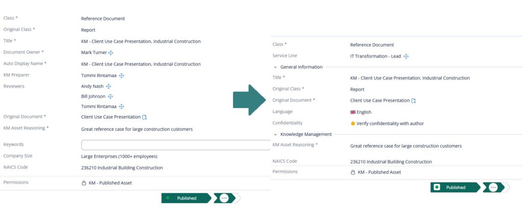 Same properties but on the right we organized them
Users scan information much faster when it is visually organized.
Additionally, sections that are not needed at a given stage can be hidden or collapsed.
Reduce decisionsEvery visible property asks the user to make a decision.
Should I fill this in?
Does this apply to my document?
What does this property even mean?
A good metadata card minimizes these decisions.
It is good practice to use:
- Automatic values
- Default values
- Value lists
- Metadata inheritance
- Calculated properties
The fewer decisions users have to make, the faster and more accurately they can classify documents.
Avoid the “Everything might be useful”One of the biggest design mistakes is trying to satisfy every department.
For instance, the Human Resources department requires three properties, the Legal department requests five more, the Finance department submits a request for four additional fields, and finally, the Compliance department adds another six.
After a few workshops, the metadata card ends up with thirty or forty properties.
Technically, everything is possible.
Practically, nobody enjoys using it.
Whenever a new property is requested, ask:
- Who will maintain it?
- Who actually uses it?
- What business process depends on it?
- What happens if it remains empty?
If there isn’t a clear answer, then the property probably isn’t necessary.
Design for the common caseMost users perform the same actions repeatedly.
Optimize the metadata card for 80% of documents rather than exceptional cases.
Advanced scenarios can reveal additional properties as needed.
Simple cases should remain simple.
Administrators often focus on configuration, whereas it is the users who interact with the interface.
Therefore, it is important to keep in mind that every additional property increases cognitive load.
Similarly, every unnecessary required field creates friction.
Conversely, every hidden property reduces complexity.
A well-designed metadata card improves not only data quality but also the user experience of the entire M-Files system.
ConclusionMetadata is one of M-Files’ greatest strengths, but only if users provide it.
The best metadata card isn’t the one that captures the most information.
Rather, it’s the one that asks the fewest questions while still collecting everything the business needs.
When users feel that the system understands their tasks instead of getting in their way, they will naturally adopt it.
Sometimes improving user satisfaction isn’t about adding new functionality; it’s about designing a better metadata card.
Whether you’re planning a new M-Files implementation or looking to improve an existing one, we can help you design a solution that is efficient, user-friendly, and aligned with your business needs. Feel free to contact us to discuss your project.
L’article Designing metadata cards that users like est apparu en premier sur dbi Blog.