Why SQL Server is confounding the Oracle Index Rebuild debate
After more than 20 years of working with Oracle databases, I have recently found myself using SQL Server for the very first time. Until now, I have been a passive observer in the My-Database-Is-Better-Than-Yours wars, so it’s a pleasant change to be able to finally contribute.
I’m pleased to report that – as a software developer – the skills map pretty well between the databases. Sure, PL/SQL and T-SQL are different languages, but most of it seems to be syntax; if you are skilled with one database then the biggest obstacle to overcome is using a new syntax, which – as IT professionals – is a pretty straightforward core skill.
Because of the similarities, I find that I can often predict SQL Server behaviour based on what I know about Oracle and I am easily lulled into a feeling of expertise with SQL Server. By far the most interesting aspect of this skill transition is when I am wrong; i.e. when I make a false assumption about SQL Server working the same way as Oracle.
- Let's discuss Index rebuilds
- Fragmentation in Oracle Indexes
- Fragmentation in SQL Server Indexes
- What about the Clustering Factor?
- Are Oracle Clusters the same as SQL Server Clustered Indexes?
- Summary
Let's discuss Index rebuilds
Index Rebuilds are a great example. One school of thought – prevalent in the SQL Server world more so than Oracle – states that indexes are like cars; they need regular servicing to keep running smoothly. In an index, “servicing” mean rebuilding. The problem – we are told – is fragmentation.
Indexes get fragmented and re-building them gets rid of fragmentation.
This is a true statement, but the underlying truth that is less frequently taught is:
Index fragmentation is not necessarily a bad thing.
Now here’s the weird bit: although there is plenty of spirited debate on this subject, the Oracle community generally agrees that index fragmentation not necessarily a bad thing, whereas the SQL Server community concludes the opposite: fragmentation is bad so rebuild your indexes.
Even more curiously, Microsoft itself recommends rebuilding fragmented indexes. But Microsoft and Oracle both use B-Tree indexes, so surely one of them is wrong, right?
Fragmentation in Oracle Indexes
Why did I specify Oracle indexes? Well, because SQL Server indexes are different. I didn’t believe it either, but I will explain later.
Both Oracle and SQL Server indexes – like a phone book – store their entries in a sorted data structure called a B-Tree (think regular indexes; we will tackle Bitmap Indexes another time). They’re pretty clever, when we want to insert a new value into the middle of the index (say, ‘M’ in the phone book), we don’t shift all of the other values to the right to make space; that would take ages. Instead, a B-Tree simply finds the block where the new entry ought to be and – if there is no spare room – it divides it into two blocks so that there is spare room. Now we have two blocks that are only half full and we can fit the new value in one of them.
Is this fragmented? Sure, but in a good way. Now there is plenty of space in both of those blocks so that the next new value doesn’t have to go through the expensive splitting process again. If we rebuild the index, it gets squashed back down and those spaces disappear. After a rebuild, just about every new value in the middle of the index will result in an expensive block split.
What if we never want to insert values into the middle of the index? Think about an index on Transaction_Date; as we create new Transactions, we use transaction dates of today, yesterday, or last week; but we almost never create a transaction for last month or last year. The index blocks that contain transaction dates older than a week will hardly ever see new values. It is wasteful to have lots of empty space in those blocks, so that’s fragmented in a bad way, right?
Well, maybe and maybe not. If we want to read just one row from one of these fragmented old blocks, then we need to read the block in which it resides. It doesn’t matter whether that block is nearly empty, half full or brimming over; we only want the one row so it’s going to cost us one whole block to get it. This sort of fragmentation would be more of a problem if we wanted to read hundreds of rows from fragmented blocks; e.g. read all the ‘M’s from the phone book. If there are fewer index entries in each block, then we need to read more blocks and this takes more time. Depending on how often we do this, it might be the sort of fragmentation we would want to fix.
Buffer Cache Impacts
It’s also worth noting the impacts on the Buffer Cache (memory), where Oracle stores recently used blocks in case they are needed again. If index blocks are denser after an index rebuild then more rows will be cached (100 full blocks in memory contain more rows than 100 half-full blocks) and queries are theoretically more likely to find any given row in the buffer cache, saving a potential disk read. In practice, this is only true if you don’t have enough memory to start with. If you already have a 90%+ buffer cache hit ratio, then you are not going to squeeze many more hits out of condensed blocks.
The much more concerning impact on the buffer cache is that when you rebuild an index, all of that index’s blocks are effectively purged from the Buffer Cache, so the very next query you perform will have to retrieve EVERY block from disk.
The Verdict
I’m not going to tell you to rebuild or not to rebuild; just understand that there are many factors at play here and you may end up making the performance worse.
For what it’s worth, the cases where I consider rebuilding are:
- Date and Sequence-allocated indexes, where new rows tend to have new values at the end of the range and there are infrequent changes to old values. Date-range partitioning can help here; you may just need to rebuild indexes on old partitions once and then leave them alone. Even without partitioning, I would only rebuild if I had SQLs with long index range scans (say 10K+ rows).
- After a big clean-up where a significant proportion of the rows have been deleted /archived and it will take months / years of normal processing to replace them.
- Bitmap Indexes and secondary indexes on Index Organized Tables are special cases that often require rebuild outside of these situations and for utterly different reasons that are beyond the scope of this article.
Oracle itself is even less detailed.
Over time, updates and deletes on objects within a tablespace can create pockets of empty space that individually are not large enough to be reused for new data. This type of empty space is referred to as fragmented free space. Objects with fragmented free space can result in much wasted space, and can impact database performance.Source: Reclaiming Unused Space
Oracle® Database Administrator's Guide
12c Release 1 (12.1)
Importantly, Oracle makes no assertions about the performance gains from rebuilding the index, or the potential scale of the performance problem that could be caused by not addressing the issue. In fact, the section in which this passage appears is about Reclaiming Unused Space, not performance.
Internal Fragmentation vs External Fragmentation
The first thing we need to get absolutely clear before talking about fragmentation in SQL Server is that the description above is actually known as Internal Fragmentation – the existence of recoverable free space within the index blocks.
Oracle separately defines External Fragmentation, which can occur when you build an index in parallel.
When you create a table or index in parallel, it is possible to create areas of free space. This occurs when the temporary segments used by the parallel execution servers are larger than what is needed to store the rows.If the unused space in each temporary segment is larger than the value of the MINIMUM EXTENT parameter set at the tablespace level, then Oracle Database trims the unused space when merging rows from all of the temporary segments into the table or index. The unused space is returned to the system free space and can be allocated for new extents, but it cannot be coalesced into a larger segment because it is not contiguous space (external fragmentation).
Source: Free Space and Parallel DDL
Oracle® Database VLDB and Partitioning Guide
12c Release 1 (12.1)
In other words, each parallel query server pre-reserves space for the index blocks it is building and – if it reserves too much – it reallocates it back to free space at the end. This can leave dozens of pockets of free space outside the index that may sit unused unless other tables/indexes grow to claim them.
In both Internal and External Fragmentation, Oracle is referring to unused space in the database that can potentially be reclaimed.
Fragmentation in SQL Server Indexes
After more than 1200 words, we finally get to the reason for this article: How SQL Server is confounding the Index Rebuild debate.
To my great surprise, Microsoft actually recommends rebuilding fragmented indexes; not just to reclaim unused space like Oracle, but also for (unspecified) performance benefits.
Heavily fragmented indexes can degrade query performance and cause your application to respond slowly.You can remedy index fragmentation by reorganizing or rebuilding an index.
Source: Microsoft Developer Network
SQL Server 2014
Reorganise and Rebuild Indexes
So Oracle does not discuss performance improvements (in fact, the consensus of the Oracle community is that – for reasons listed above – regular index rebuilds may actually degrade performance), yet Microsoft comes right out and recommends rebuilding fragmented indexes for performance gains. Who is right?
My initial assumption – a false one – was that Microsoft had just signed up to an antiquated practice that was born in a time when memory was scarce and block density was a much more important consideration.
The reality is that Microsoft defines Fragmentation differently. I have been a bit disingenuous with the quote above; here is the preceding paragraph that I omitted:
The SQL Server Database Engine automatically maintains indexes whenever insert, update, or delete operations are made to the underlying data. Over time these modifications can cause the information in the index to become scattered in the database (fragmented). Fragmentation exists when indexes have pages in which the logical ordering, based on the key value, does not match the physical ordering inside the data file.Source: Microsoft Developer Network
SQL Server 2014
Reorganise and Rebuild Indexes
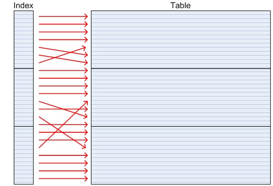
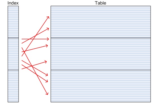
This is key: in SQL Server, fragmentation is about the ordering of pages (blocks), not free space in those pages (Oracle’s Internal Fragmentation) or free space outside of the index (Oracle’s External Fragmentation).
Now if you are reading this and saying to yourself, “Aha! Oracle calls that Clustering Factor!” then you can stop. It’s not. The Clustering Factor in Oracle indexes refers to the likelihood that rows which are neighbours in the index will also be neighbours in the underlying table; the logical sequencing of blocks in the index can still be scattered. Let’s come back to clustering factors later.
SQL Server fragmentation simply means that when you get to the end of one page, how likely is it that the next logical value in the index (i.e. if you are reading the index in ascending order) is in the very next physical block on disk.
I thought that I must have misunderstood this the first time I read it; how could that even be important? If you read a block (page) from the index and then go back and do something with it (like table lookups), what is the likelihood that the hard disk is still sitting where you left it when you come back? I mean, I can see the advantage in having the disk head positioned perfectly for the next read, but in a modern multi-processor, time-sharing operating system with databases on striped and mirrored network disk farms that are shared with other servers … well, I just can’t see the point.
My first Oracle job in 1990 was coding SQL*Forms 2.3 on an Oracle 5.1b database under Microsoft DOS 3.3. Since DOS was not a time-sharing OS, your computer only did one thing at a time; so you could spend as long as you like between disk reads and the disk head will be where you left it. But how could that possibly work on modern database servers?
I was curious enough to have a go at debunking the SQL Server fragmentation “myth”; I just couldn’t see how physical sequencing of blocks/pages in an index could have any significant material impact that would warrant rebuilding the index. Part of this was my Oracle bias; Oracle just doesn’t care about physical sequencing of blocks in the index, so why should SQL Server?
To my chagrin, I ended up … bunking? … the “myth”. I bunked it to the point that I can confirm that it is not actually a myth; matching the physical and logical sequence of blocks/pages in a SQL Server index really can have a material performance impact … to some types of queries.
Test case – SQL Server Fragmentation
Since this is an Oracle blog, I’m not going to go into a lot of detail about my test case, but I set up two Clustered Indexes (bit like an Index Organized Table) with approximately the same level of internal fragmentation; one was perfectly sequenced (0% SQL Server fragmentation) and one was almost perfectly fragmented (97% SQL Server fragmentation).
Then I ran the following four tests:
- Test 1: Random reads: From each table, I looked up one million unique rows in a random sequence. This mimics the behaviour of many OLTP applications, which perform frequent, unordered, single row reads. Result: no difference between the fragmented and sequenced indexes.
- Test 2: Sequential single row reads: From each table, I looked up one million unique rows in sequence, but only one at a time. This is the type of behaviour you might get running a SQL inside a (sorted) cursor loop. In both cases, SQL Server performs a lookup on the first row in the page resulting in a disk read; then subsequent reads use the page in cache. When we go to find the next index page, the sequenced index will find it right next door, whereas the fragmented index will find it elsewhere on disk. I had nothing else running on my quad-core hyper-threaded Win7 laptop, so I wasn’t terribly surprised to see a performance advantage for the sequenced index, although I was surprised to see it as high as 40%. I’m not going to read too much into this result as the scenario is a bit contrived: I cleared the database cache by restarting the database before each run, but I didn’t clear the physical disk cache. Under a real production scenario, the database cache would not be empty, so I’m not going to waste a lot of time explaining a 40% improvement to a ‘perfect storm’ of disk reads.
- Test 3: Fast Full Scan: Microsoft calls it a Seek when you read an index using a key, or a Scan when you do a full pass of the index without using the key, so a SQL Server Index Scan is like Oracle’s Fast Full Scan. The sequenced index was almost twice as fast for reasons I cannot adequately explain. I assume that the SQL Server Index Scan would read the index in physical order (not logical order) and that there is no real advantage to physically sequencing the rows. Either this assumption is wrong, or my test case was imperfect and there were differences between the tables other than fragmentation.
- Test 4: Range Scan: Starting at some point in the index, I read one million consecutive rows using a SQL Server Index Seek (i.e. an Index Range Scan in Oracle). After processing the last row in the page, the sequenced index would find the next block right next door, but the fragmented example would find the next page somewhere else on disk. Logically, this was the same as Test 2, except it was done in a single statement, not a series of single-row lookup. For this reason I expected the same result; so how surprised was I to see the sequenced index perform ten times faster than the fragmented index? Pretty damned surprised, I can tell you.
Discovery! Why Index Rebuilds (sometimes) improve performance in SQL Server
The secret of success in Test Case 4 above for a well sequenced SQL Server index (low fragmentation) is multi-block reads; known in SQL Server as “Read Ahead”.
In Oracle, Full Table Scans and Fast Full Index Scans read the entire table/index from start to finish, but they do it many blocks at a time. The Oracle initialization parameter DB_FILE_MULTIBLOCK_READ_COUNT defines how many blocks to read at a time in Full Table Scans / Fast Full Index Scans, and it is common – especially with non-parallel queries on network disk – for multi-block reads to out-perform single block reads by an order of magnitude.
Oracle’s Index Range Scan will read indexes in logical order (not physical) and will always perform single block reads. I wrongly assumed that the same was true for SQL Server and that was my downfall. In fact, SQL Server does something quite clever; based on the query and the table/index statistics, it estimates how many blocks will be read in a Non-Unique Seek (Range Scan) operation and then – depending on the fragmentation of the index – it determines whether it will be advantageous to read-ahead in the index.
For example, if the statistics suggest that a query will return 10K rows and the index contains (on average) 100 rows per page, then it estimates the query will need 100 pages from the index. If the fragmentation of the index is (say) 3%, then it is a reasonable assumption that – after looking up the first page of matching rows in the index – the following 100 pages will contain 97% of the target rows, leaving only 3% to go and find using single page reads. Such a query can probably be resolved with fewer than 10 round trips to the disk; compare that to the 100 round trips performed by single-block reads and we see where the 10x performance gain comes from.
So does this translate to Oracle?
Short answer: no. When Oracle reads indexes in logical order (e.g. Range Scans), it always does so using single-block reads. Without the advantage of multi-block reads, there is only marginal advantage in physically sequencing an index.
To demonstrate, let’s build a test case that performs range scans of a well-sequenced index vs. a poorly sequenced index (i.e. “fragmented” as defined by Microsoft SQL Server). To eliminate any noise created by the table underlying the index, we will use an Index Organized Table. Incidentally, this test case is nearly identical to the method I used to discover the “Read Ahead” behaviour in well-sequenced SQL Server indexes.
To create the “fragmented” (or poorly sequenced) table, we will insert rows into the table in a pseudo-random order. This will cause blocks to split when they are full, with new blocks allocated at the end of the segment rather than being adjacent to and in sequence with blocks having neighbouring values.
-- FRAGTEST is an Index Organized Table
-- Rows are created in order of ascending values of "n"
-- but indexed on the numerical reverse of that number
-- stored as column "r"
-- eg. Rows 11, 12, and 13 will be created in that order but
-- indexed as 1100000, 2100000 and 3100000
-- Column "filler" is just there to take up space and reduce
-- the block density.

CREATE TABLE fragtest (
  n NUMBER(12)
, r NUMBER(12) PRIMARY KEY
, filler VARCHAR2(80)
) ORGANIZATION INDEX TABLESPACE BIG
/


DECLARE
    i INTEGER := 0;
    batchsize INTEGER := 1000;
BEGIN
    FOR i IN 0 .. 10000 LOOP
        INSERT INTO fragtest
        SELECT n
        ,      TO_NUMBER(REVERSE(TO_CHAR(n, '0999999'))) AS r
        ,      LPAD(TO_CHAR(n), 80, TO_CHAR(n))
        FROM (
            SELECT i * batchsize + level - 1 AS n
            FROM dual
            CONNECT BY LEVEL <= batchsize
        );
        COMMIT;
    END LOOP;
END;
/
I’m testing this on a virtual machine and boy is it slow with every row being inserted into a different block. I didn’t actually let it finish creating the full 10M rows, stopping it at around 3.7M. I “tested” the results using a SELECT * query, which performed a FAST FULL INDEX SCAN and displayed the rows in stored order. The first 70 or so rows were all for ordered values of “r” between 5000000 and 5000192 and then the next 70 or so were all order values of “r” between 4700000 and 4700192. i.e. The values within each block were ordered, but the blocks themselves were not ordered
For the defragged table, I created the same table in a single statement (which will pre-sort the data in TEMP), except I used the column “n” as the primary key. Since rows were inserted in order, blocks were never split and new blocks were allocated with increasing values of “n”. Not surprisingly, this one ran a lot faster. Also not surprisingly, it had a much higher block density (more rows per block), so to get a comparable block density to the fragmented example, I created twice as many rows and then deleted all of the odd values of “n”. The result was not a perfect match for the block density of the fragmented table, but it was close enough for demonstration purposes.
I also “tested” this table using a FAST FULL INDEX SCAN to display the rows in stored order. It started with n = 0, 2, 4 and climbed from there, so I conclude that it was perfectly defragmented (using the SQL Server definition).
DEFINE batchsize=1000

CREATE TABLE defragtest (
 n  PRIMARY KEY
, r
, filler
) ORGANIZATION INDEX TABLESPACE BIG PCTFREE 10
AS
SELECT  n
,      TO_NUMBER(REVERSE(TO_CHAR(n, '0999999'))) AS r
,      LPAD(TO_CHAR(n), 80, TO_CHAR(n))
FROM (
    SELECT i * &batchsize + lvl - 1 AS n
    FROM (
        SELECT level AS lvl
        FROM dual
        CONNECT BY LEVEL <= &batchsize
    ) a
    CROSS JOIN (
        SELECT level - 1 AS i
        FROM dual
        CONNECT BY LEVEL <= 3708 * 2
    )
)
/

DELETE FROM defragtest
WHERE MOD(n,2) = 1;
First of all, let’s benchmark multi-block reads, which we expect to be much faster than single block reads. In the head-to-head tests below we will perform single block reads over 740K rows, so let’s make the benchmark a FAST FULL INDEX SCAN (multi-block reads) over the same number of rows.
SQL> select count(*)
  2  from fragtest
  3  WHERE rownum <= 740000;

  COUNT(*)
----------
    740000

Elapsed: 00:00:01.52

----------------------------------------------------
| Id  | Operation              | Name              |
----------------------------------------------------
|   0 | SELECT STATEMENT       |                   |
|   1 |  SORT AGGREGATE        |                   |
|*  2 |   COUNT STOPKEY        |                   |
|   3 |    INDEX FAST FULL SCAN| SYS_IOT_TOP_74583 |
----------------------------------------------------

Statistics
----------------------------------------------------------
        154  recursive calls
          0  db block gets
      18335  consistent gets
      18382  physical reads
          0  redo size
        422  bytes sent via SQL*Net to client
        415  bytes received via SQL*Net from client
          2  SQL*Net roundtrips to/from client
          6  sorts (memory)
          0  sorts (disk)
          1  rows processed
So there’s out benchmark: 740K rows (18.5K blocks) in 1.52 seconds.
Now for the head-to-head: here is a test run of 740K rows selected in a range scan from each Index Organized Table. With similar block densities, they perform about the same number of physical reads (18-20K) and take about the same amount of time.
First: the “defragmented” table.
SQL> SELECT count(*)
  2  FROM defragtest
  3  WHERE n BETWEEN 1000000 and 2482000;

  COUNT(*)
----------
    741001

Elapsed: 00:00:04.72

-----------------------------------------------
| Id  | Operation         | Name              |
-----------------------------------------------
|   0 | SELECT STATEMENT  |                   |
|   1 |  SORT AGGREGATE   |                   |
|*  2 |   INDEX RANGE SCAN| SYS_IOT_TOP_74615 |
-----------------------------------------------

Statistics
----------------------------------------------------------
          0  recursive calls
          0  db block gets
      20877  consistent gets
      20877  physical reads
          0  redo size
        424  bytes sent via SQL*Net to client
        415  bytes received via SQL*Net from client
          2  SQL*Net roundtrips to/from client
          0  sorts (memory)
          0  sorts (disk)
          1  rows processed
Now the fragmented table. Note that the SQL selects a different range of values because the columns “r” (primary key on the fragmented table) and “n” (primary key on the defragmented table) are constructed differently. Importantly, both examples read about the same number of rows, as evidenced by the results of the COUNT.
SQL> select count(*)
  2  from fragtest
  3  where r between 1000000 and 3000000;

  COUNT(*)
----------
    741801

Elapsed: 00:00:04.27

-----------------------------------------------
| Id  | Operation         | Name              |
-----------------------------------------------
|   0 | SELECT STATEMENT  |                   |
|   1 |  SORT AGGREGATE   |                   |
|*  2 |   INDEX RANGE SCAN| SYS_IOT_TOP_74583 |
-----------------------------------------------

Statistics
----------------------------------------------------------
          0  recursive calls
          0  db block gets
      18408  consistent gets
      18408  physical reads
          0  redo size
        424  bytes sent via SQL*Net to client
        415  bytes received via SQL*Net from client
          2  SQL*Net roundtrips to/from client
          0  sorts (memory)
          0  sorts (disk)
          1  rows processed
Prior to the test, I flushed the buffer cache so that all data would need to be read from disk. I ran this test several times with similar results.
Conclusion: The FAST FULL INDEX SCAN was clearly much faster (about 3x) than either INDEX RANGE SCAN, however the two INDEX RANGE SCANS – one fragmented and one not fragmented – performed about the same. Unlike SQL Server, Oracle clearly does not take advantage of a nicely sequenced index to perform multi-block reads during a long range scan.
What about the Clustering Factor?
OK, so Oracle identifies Fragmentation as an opportunity to reclaim unused space, whereas SQL Server identifies it as a performance problem that can be fixed with an index rebuild. But that’s because they define Fragmentation differently.
That SQL Server definition of Fragmentation – where the physical order of pages (blocks) matches the logical order in the index – sounds a bit like Oracle’s Clustering Factor. How is it different?
Let’s be completely clear: Clustering Factor has nothing to do with Fragmentation (regardless of whether we are using Oracle’s or Microsoft’s definition). Whereas Microsoft Fragmentation is something that describes the index in isolation, Clustering Factor describes the relationship between an Index with its underlying table.
Consider the following table:
CREATE SEQUENCE my_seq;

CREATE TABLE my_table (
    id          NUMBER(12) DEFAULT my_seq.NEXTVAL PRIMARY KEY
,   description VARCHAR2(200)
);
Assuming we never delete or update rows in MY_TABLE, blocks will be allocated to the table in physical order and rows will be added with increasing values of the column ID. E.g. The first block might contain ID values of (say) 1 to 30, then the second block would contain 31-60, and the third block 61-90, etc.
In the PRIMARY KEY index, all of the values in any given leaf block will be sorted. Note that we are just talking about the contents of a single index block; logically sequential blocks may still be scattered in the index (i.e. “fragmented” in SQL Server). Say a single index block contains ID values 1 to 300; if we were to read these rows in a RANGE SCAN, we would go looking for ID=1 in the table and find it in the first block, which we may need to read from disk if it has not been recently used. When we look for the block containing ID=2, 3, 4 etc, we find that they are in the same block as ID=1, which is currently in the buffer cache and therefore quick to find.
Such an index is said to have a low clustering factor. A low clustering factor means that keys that are adjacent in the index are likely to be co-located in the same block in the table. When we perform a range scan of such an index, we get a very high buffer cache hit ratio.
generally point to neighbouring rows in the table.
If rows for ID=1, 2, 3 etc were all in different blocks in the table then the PRIMARY KEY index would have a high clustering factor. A range scan of such a table would read and cache the block for ID=1, and then when it looks for the block with ID=2, it may need to read it from disk because it is in a different block. In the worst case, rows ID = 1 .. 30 might be in 30 different blocks, so a range scan of an index with very high clustering factor (i.e. scattered in the table) may cost as many as 30 physical reads, whereas an index with a very low clustering factor (i.e. ordered in the table) may cost just a single block read from disk.
generally do not point to neighbouring rows in the table.
It’s time for a test case. Let’s create a table with two indexes: one with a high clustering factor and one with a low clustering factor.
CREATE TABLE clusttest (
  n NUMBER(12)
, r NUMBER(12)
, filler VARCHAR2(80)
) TABLESPACE BIG
/

-- Insert 10,000,000 in increasing values of N with scattered
-- values of R

DECLARE
    i INTEGER := 0;
    batchsize INTEGER := 1000;
BEGIN
    FOR i IN 0 .. 9999 LOOP
        INSERT INTO clusttest
        SELECT n
        ,      TO_NUMBER(REVERSE(TO_CHAR(n, '0999999'))) AS r
        ,      LPAD(TO_CHAR(n), 80, TO_CHAR(n))
        FROM (SELECT i * batchsize + level - 1 AS n FROM dual CONNECT BY LEVEL <= batchsize);
        COMMIT;
    END LOOP;
END;
/


-- This index will have a low clustering factor, meaning
-- that neighbouring rows in the index will frequently be
-- neighbouring in the table

CREATE UNIQUE INDEX clusttest_n
ON clusttest (n) TABLESPACE BIG;

-- This index will have a high clustering factor, meaning
-- that neighbouring rows in the index will frequently NOT be
-- neighbouring in the table

CREATE UNIQUE INDEX clusttest_r
ON clusttest (r) TABLESPACE BIG;

-- Gather statistics

EXEC DBMS_STATS.GATHER_TABLE_STATS(USER, 'CLUSTTEST');

  1  select index_name, clustering_factor
  2  from user_indexes
  3* where table_name = 'CLUSTTEST'

INDEX_NAME                     CLUSTERING_FACTOR
------------------------------ -----------------
CLUSTTEST_R                              9763622
CLUSTTEST_N                               165147
So now we have two unique indexes on the same table. The index on column R is highly scattered in the table; i.e. values that occupy the same index block tend not to occupy the same table block. The index on column N has a much lower clustering factor, so rows that occupy the same index will much more often occupy the same table block.
Now we benchmark a SQL on each table. Note in these examples that I am using a hint to enforce the index range scan; especially for the example with the high clustering factor, Oracle knew that a long range scan was a bad idea and was choosing a full table scan instead.
First: column N (low clustering factor).
  1  SELECT /*+ INDEX(clusttest) */ MAX(filler)
  2  FROM   clusttest
  3* WHERE  n BETWEEN 1000000 AND 1100000

MAX(FILLER)
--------------------------------------------------------------------------------
11000001100000110000011000001100000110000011000001100000110000011000001101100000

1 row selected.

Elapsed: 00:00:00.43

------------------------------------------------------------
| Id  | Operation                    | Name        | Rows  |
------------------------------------------------------------
|   0 | SELECT STATEMENT             |             |     1 |
|   1 |  SORT AGGREGATE              |             |     1 |
|   2 |   TABLE ACCESS BY INDEX ROWID| CLUSTTEST   |   100K|
|*  3 |    INDEX RANGE SCAN          | CLUSTTEST_N |   106K|
------------------------------------------------------------

   3 - access("N">=1000000 AND "N"<=1100000)


Statistics
----------------------------------------------------------
       1578  consistent gets
       1578  physical reads
And now for column R (high clustering factor – expected to be slower):
  1  SELECT /*+ INDEX(clusttest) */ MAX(filler)
  2  FROM   clusttest
  3* WHERE  r BETWEEN 1000000 AND 1100000

MAX(FILLER)
--------------------------------------------------------------------------------
99999019999901999990199999019999901999990199999019999901999990199999019999999901

1 row selected.

Elapsed: 00:01:14.30

------------------------------------------------------------
| Id  | Operation                    | Name        | Rows  |
------------------------------------------------------------
|   0 | SELECT STATEMENT             |             |     1 |
|   1 |  SORT AGGREGATE              |             |     1 |
|   2 |   TABLE ACCESS BY INDEX ROWID| CLUSTTEST   |   100K|
|*  3 |    INDEX RANGE SCAN          | CLUSTTEST_R |   100K|
------------------------------------------------------------

   3 - access("R">=1000000 AND "R"<=1100000)


Statistics
----------------------------------------------------------
     100227  consistent gets
     100227  physical reads
So, there we have it: two almost identical execution plans but vastly different outcomes. The more clustered index (low clustering factor) completed in less than half a second with about 1500 physical reads from disk, whereas the less clustered index (high clustering factor) completed in over a minute (more than 100 times longer) with over 100K physical reads (20 times more IO).
How can we improve the Clustering Factor?
So if the Clustering Factor is so gosh-darned important for long range scans like those in the examples above, is there anything we can do to improve it?
I have sometimes heard it suggested that rebuilding the index will improve the clustering factor. Perhaps these are SQL Server programmers getting the Clustering Factor confused with SQL Server Fragmentation, because it is not true; when you rebuild the index, it will still be in the same order and so will the table. You cannot influence the order of rows in the index; but you can influence the in order of rows in the table.
There are four good ways to control the Clustering Factor of an index, but note this: you can only control ONE index on a table. Once you organise the table based on that index key, you will impact the Clustering Factor of all other indexes, potentially impacting the Buffer Cache hit ratio or (more likely) ruining the performance of some other long range scan.
- Rebuild the table, sorting the rows as you insert them so that they are loaded in the same order as the index key. EDIT: As of Oracle 12.1.0.2, the Attribute Clustering feature allows us to define columns that will be used to cluster rows with like values whenever the table or partition is rebuilt, thereby simplifying this process.
- For Data Warehouse applications, sort the rows in the order of the index key before you load them. In this way, rows inserted in the same load will be clustered, although rows loaded at different times will not be clustered. EDIT: As of Oracle 12.1.0.2, the Attribute Clustering feature allows us to define columns that will be used to cluster rows loaded via Direct Path or partition MOVE, MERGE, SPLIT and COALESCE operations.
- Consider the possibility of an Index Organized Table. By storing the entire table in a B-Tree index structure, queries that use the Primary Key index will never have to do a table lookup. Note that there is a cost: queries on secondary indexes (non primary key) will be considerably slower and secondary indexes may need regular maintenance to stay efficient. If you are in ANY doubt, consult your DBA. If you are still in doubt, do some benchmarking that involves production-like levels of updates on the table. If you are still in doubt, don’t use Index Organized Tables.
- Consider the possibility of a Clustered Table using either an Index Cluster or a Hash Cluster. A table stored in an Oracle cluster will co-locate rows with the same key in the same block. There will also be maintenance and storage considerations for Clusters, so the same disclaimers as for Index Organized Tables apply. Never implement an Oracle Cluster without discussing it with your DBA.
Also note that if you do decide to rebuild a table (option 1), you will only be reorganising existing rows; new rows created afterwards will continue to load in an un-clustered manner.
Here is an example of re-clustering a table:
RENAME clusttest TO clusttest_old;

CREATE TABLE clusttest AS
SELECT *
FROM   clusttest_old
ORDER BY r
/

DROP TABLE clusttest_old PURGE;


CREATE UNIQUE INDEX clusttest_n
ON clusttest (n) TABLESPACE BIG;

CREATE UNIQUE INDEX clusttest_r
ON clusttest (r) TABLESPACE BIG;

EXEC DBMS_STATS.GATHER_TABLE_STATS(USER, 'CLUSTTEST');

  1  SELECT index_name, clustering_factor
  2  FROM user_indexes
  3* WHERE table_name = 'CLUSTTEST'

INDEX_NAME                     CLUSTERING_FACTOR
------------------------------ -----------------
CLUSTTEST_R                               157071
CLUSTTEST_N                             10300555
Note that I used an ODER BY when I recreated the CLUSTTEST table; this time the rows are ordered by column R instead of column N. Also note that the Clustering Factors of the two indexes have been reversed; the index on column R is now the one with low clustering factor.
So what does SQL Server say about Clustering Factor?
Interestingly, I cannot find a SQL Server equivalent to Oracle’s Clustering Factor. But that doesn’t mean Microsoft thinks it is unimportant; quite to the contrary, Microsoft considers it so important that they enshrine one and only one index on the table as the Clustered Index and bestow it with even greater powers than Oracle (hard to believe, I know!).
The term “Clustered Index” in SQL Server is actually misleading; it is in fact the table that is clustered. When you create a Clustered Index on a SQL Server table, it rebuilds the table in the form of a B-Tree index. In this way, it is analogous to Oracle Index Organized Table, although it is not subject to the same issues as IOTs with regards to secondary (non-clustered) indexes, making them much more versatile. So much so, Microsoft recommends that almost every table should be clustered:
With few exceptions, every table should have a clustered index. Besides improving query performance, a clustered index can be rebuilt or reorganized on demand to control table fragmentation.
Source: Microsoft Developer Network
SQL Server 2014
Create Clustered Indexes
The big difference between a SQL Server Clustered Index and an Oracle index with a low Clustering Factor is that the Oracle index will still need to perform table lookups, whereas SQL Server stores the table in the Clustered Index so you never need to perform a table lookup.
Are Oracle Clusters the same as SQL Server Clustered Indexes?
Short answer: no. As discussed above, a Clustered Index in SQL Server actually rebuilds the table as a B-Tree. This is very much like an Oracle Index Organized Table, but not like a Cluster.
A Cluster in Oracle is little more than a table that pre-reserves space in blocks for new rows with the same key values as existing rows. With a regular (heap organized) table, Oracle will keep inserting rows into any block with free space until it is full and then move on to another block with no regard for the incoming row or the rows already in the block.
Oracle supports two types of Table Clusters: Index Clustered Tables (or Indexed Cluster) and Hash Clustered Tables (or Hash Cluster). With an Indexed Cluster, if the new row shares the same cluster key as an existing row, then Oracle will try to insert it into the same block, otherwise it will allocate a brand new block. An Indexed Cluster has a completely separate B-Tree structure called the Cluster Index that functions exactly like a regular index to find rows in the Indexed Cluster.
With a Hash Cluster, there is no Cluster Index. Instead, the cluster key is hashed to a number that is translated to an address in the table. In this way, you can run a query with (say) WHERE keyval = 13 and go straight to the block containing keyval=13 without having to lookup an index. With hash clusters, you specify the total number of hash keys and the amount of space to reserve for each hash key. In this way, you can use a single block to store rows with different cluster key values – this is not possible with an Indexed Cluster.
Oracle can also store multiple tables in the same cluster. For example, if you had tables INVOICE and INVOICE_LINE then you could create a single cluster containing both tables using the cluster key of INVOICE_NUMBER. All rows from both tables having the same INVOICE_NUMBER will be stored in the same block. This can make for extremely efficient joins.
Does SQL Server have Table Clusters like Oracle?
No. There would hardly be any point; for a single table it would not perform as well as a SQL Server Clustered Index, and for a multi-table cluster there would probably be very few cases that would deliver a measurable and worthwhile performance advantage over Clustered Indexes.
In fact, Oracle’s hash joins and memory management are now so refined that there are very few situations where Table Clusters can offer a compelling performance advantage.
Why doesn’t Oracle have Clustered Indexes?
Well it does … kind of. Index Organized Tables are the same as a SQL Server Clustered Index in that they are both tables that are stored in a B-Tree index structure.
The key advantage of Oracle’s IOTs is that you can specify some infrequently used columns that are stored outside of the B-Tree so that you get more rows per block. Queries (especially long range scans) that don’t use those ‘overflow’ columns can be faster because you read fewer blocks to get the same number of rows. Queries that do use the ‘overflow’ columns are slower because they have to go and lookup the overflow structure.
The key advantage of SQL Server Clustered Indexes is their implementation of secondary indexes. Oracle indexes find a row in the underlying table via an absolute address called a ROWID. Every ROWID contains the physical location of the block, so it is quite efficient to find a row in table once you have a ROWID; you just go straight to the block and read it.
IOTs are different because – when blocks in the B-Tree become full and are split – some rows are migrated to new addresses, so any address that is stored in a secondary index would be invalidated. Instead, Oracle uses a process called a ‘Physical Guess’, which is as dodgy as it sounds. When searching via a secondary index in an IOT, if the Physical Guess is wrong then Oracle will need to follow the chain of index leafs until it finds the actual location of the row. In an IOT that is subject to many INSERTS and UPDATES, the Physical Guesses will grow stale quickly and the secondary index will need to be rebuilt.
In contrast, Non-Clustered Indexes on a Clustered SQL Server table do not use ROWIDs; they use the Cluster Key (usually also the Primary Key) to locate rows in the Clustered Index. The process for looking up a row via a Non-Clustered Index in SQL Server is:
- Navigate the B-Tree of the Non-Clustered index looking for a given key value.
- Retrieve the Cluster Key value from the leaves of the Non-Clustered Index.
- Use the Cluster Key to navigate the B-Tree of the Clustered Index, finding the table row stored in the Clustered Index.
Although this process seems more cumbersome than Oracle’s ROWID for normal (heap organized) tables, it has a distinct advantage over Oracle’s Index Organized Tables because secondary indexes do not need to be regularly rebuilt to maintain the accuracy of Physical ROWID Guesses.
Summary
So, where does that leave us in the Index Rebuilding debate? Let’s summarise:
- Internal Fragmentation is when the natural process of maintaining a table leaves recoverable space in index blocks. In Oracle, we may rebuild these indexes to recover that space if we think it will not be used by newly inserted rows, but there may be positive and negative performance impacts.
- External Fragmentation (in Oracle) is when there are pockets of unusable space in database files that are not used by any table or index. Far from fixing the problem, parallel index rebuilds are the primary cause of the problem. It can be fixed by reorganizing (coalescing) the tablespace, or avoided altogether by using uniform extent sizes. External fragmentation does not cause performance problems.
- SQL Server’s definition of Fragmentation is different to Oracle. It occurs when the physical order of leaf pages (blocks) in the index does not match the logical order of the index key. It does not significantly impact performance of unique lookups or full index scans, but it does have a significant performance impact on long range scans (non-unique seek in SQL Server) because it thwarts multi-page reads. Regular index rebuilds may be beneficial in SQL Server to maintain performance of long range scans. Oracle does not do multi-page reads on range scans, so the logical vs. physical order of blocks in the index has no impact.
- Oracle’s Clustering Factor has a significant impact on the performance of long index range scans. The Clustering Factor of just one index on a table can be improved – not by rebuilding the index – but by rebuilding the table in a sorted order. Such a table rebuild will also necessitate index rebuilds, which may have both positive and negative impacts on other types of queries.
- Oracle Clusters are not the same as SQL Server Clustered Indexes. Many of the benefits of Oracle Clusters have been diluted over the years by better memory management and the introduction of Hash Joins. Today, they are rarely used.
- Oracle Index Organized Tables are similar to SQL Server Clustered Indexes, but they are very specialized due to the maintenance and performance costs of secondary indexes, whereas SQL Server Clustered Indexes are ubiquitous.
So, should we rebuild indexes? Well, it depends…
- rleishman's blog
- Log in to post comments
Comments
Low and High clustering factor - new definition
Ross,
Very nicely explained. I like the clustering factor part, beatifully explained in simple terms without JARGONS.
So, I am going to steal this from you, my new definition for clustering factor in Oracle :
Higher the matching of order of physical blocks to the logical order in the index, lower is the clustering factor, and vice-versa.
Regards,
Lalit
Indexing: SQL Server v Oracle
First, I have to say that Ross's latest article here may be the best exposition of indexing with regard to rebuilds that I have ever read. It is on a par with his series on bitmap indexes The Bitmap Conspiracy
I can perhaps contribute one point. Some years ago when teaching an Oracle DB tuning class, one student who did a lot of work with SQL Server placed great emphasis on the power of reverse key indexes. The way she described it (if I understood her correctly) was that SQL Server databases have a massive problem with concurrency. Microsoft's best practice is always to co-locate data items that might be accessed together or consecutively, the idea being that this means the data blocks will be cached in memory. Apparently, a lot of SQL Server tuning is oriented towards this. The clustered index is a perfect example. But this means that in a multi-user environment you may have dreadful problems with what we would call "buffer busy wait" because concurrent inserts to a table all hit the same block, as do inserts of consecutive values into an index. This is a major factor in SQL Server scalability issues: you cannot distribute concurrent access across many blocks.
Oracle provides two facilities that address this problem. Reverse key indexes will spread consecutive key inserts across the full width of the index, and hash clusters will distribute concurrent table inserts throughout the whole cluster. With regard to index clustering factor, of course use of reverse key indexes or hash clustered tables will destroy any relationship between the ordering of the keys and the ordering of the table. But for high load concurrent insert, this is often what is required.
--
John Watson
Oracle Certified Master DBA
http://skillbuilders.com
Concurrency and hot blocks
Kind words, John. Thank you.
Between this article and a few others I have written on indexes, I have never really explored reverse key indexes. It's probably because I don't feel qualified; I now work almost exclusively in the Data Warehouse space where concurrent DML is only a consideration for the ETL and therefore easily controlled by the ETL application. Also, because of the nature of the problem, it is terribly difficult to set up a plausible test case without using a genuine production workload on Oracle Real Application Testing - Database Replay (something to which I don't have access). As you alluded, if you did set up such a test case, you would need to demonstrate that you have not only solved the hot block problem, but that you haven't created more issues with respect to Clustering Factors.
I had never considered using Clusters to solve a hot block problem, although I suppose that they could. I don't see why it should be limited to Hash Clusters though; I expect Index Clusters would work just as well, but you would need an appropriate Cluster Key that suited the one-key-per-block restriction. But to me it feels counter intuitive to use Clusters to SEPARATE rows that have a common bond (the time they were inserted) because clusters are all about keeping rows together that share a common bond (the cluster key). I am very wary of using a feature to capitalise on a SECONDARY benefit if you are not using the primary benefit (eg. avoiding globally partitioned indexes because locally partitioned indexes are easier to manage). All too often I see unforeseen and undesirable side-effects (eg. using my previous example, PARTITION RANGE ALL range scans for a highly selective index key).
Attribute Clustering 12.1.0.2
I have just made some edits regarding Attribute Clustering, a new feature of 12.1.0.2 that can be used to improve Clustering Factors in a declarative fashion during Direct Path Load, segment rebuild, or partiion management operations.