

Randolf Geist
Oracle 19c RU Release Update 19.19 nice little enhancement: DBA_HIST_SQL_PLAN ACCESS_PREDICATES and FILTER_PREDICATES columns populated
I've recently found out by coincidence a nice little enhancement that apparently was introduced with the 19.19 Release Update - a backport of the fix that was originally introduced with Oracle 20c / 21c populating the ACCESS_PREDICATES and FILTER_PREDICATES columns in DBA_HIST_SQL_PLAN.
This fix is truly a long awaited one - in fact the problem originally came from an ORA-600 error / bug in Oracle 9i (!) when populating execution plans in STATSPACK if I remember correctly, the workaround back then was setting the parameter "_cursor_plan_unparse_enabled" to FALSE which resulted among other things in those columns not being populated. This had been carried forward to AWR when it was originally implemented in Oracle 10g.
The original bug / root cause was fixed a very long time ago (although there is for example bug ORA-600 [qksxaCompactToXml:2] When Generating An Execution Plan (Doc ID 1626499.1) which applies to Oracle 11.2 fixed in 12.1) but in all that time Oracle never managed to enhance the AWR code to include those columns again when populating DBA_HIST_SQL_PLAN.
When Oracle 20c / 21c came out Oracle finally included the fix.
And now - although it is not part of the official documentation listing the new features added to 19c Release Updates (which also misses at least the backport of Automatic SQL Tuning Sets to Oracle 19.7 RU) - according to MyOracleSupport document Missing FILTER_PREDICATES And ACCESS_PREDICATES In DBA-HIST_SQL_PLAN (Doc ID 2900189.1) this has been backported to the 19.19 RU.
I currently only have access to the 19.20 RU, so I can't confirm that it's already there in 19.19 but in 19.20 definitely those columns in DBA_HIST_SQL_PLAN are populated (and in 19.16 they definitely don't get populated) - so this is very good news for those that regularly deal with execution plan details.
Without the ACCESS_PREDICATES and FILTER_PREDICATES it's not possible to fully understand the meaning of an execution plan - for example you can't tell how efficient an index access path is (are there FILTER predicates on index access operation level in addition to the ACCESS predicates indicating a suboptimal usage of the index), you might not be able to tell if a HASH JOIN includes additional FILTER predicates (potentially eating up a lot of CPU), you might not be able to fully understand the shape of an execution plan because you don't see what actually happens as part of a FILTER operation to just name a few cases where those columns are crucial for understanding / assessing properly an execution plan.
Oracle 21c / 23c New Features - move a partitioned table in a single command
Just a quick note about a nice little enhancement that might have gone unnoticed so far - since 21c it's now possible to move all partitions and subpartitions of a partitioned heap table using a single ALTER TABLE MOVE command.
So before 21c - if you had a (sub)partitioned heap table and tried to do:
ALTER TABLE <PART_TABLE> MOVE ...
then you got the error message "ORA-14511: cannot perform operation on a partitioned object" and you had to move each physical segment separately - so for a composite partitioned table this was only allowed on subpartition level, for partitioned tables on partition level.
Now from 21c on this is possible and also officially documented here and here for example.
Note that it looks like that it is still not supported to move a partition in case the table is subpartitioned - this still throws the error message "ORA-14257: cannot move a partition which is a composite partition" - so the feature at present is limited to moving the entire table on global level.
However, what is still not possible - even in 23c (FREE) - rebuilding a (sub)partitioned index using a single command.
So running:
ALTER INDEX <PART_INDEX> REBUILD ...
on a (sub)partitioned index still throws the error message: "ORA-14086: a partitioned index may not be rebuilt as a whole", which is a pity - and leaves you again only with the option to perform the rebuilds on the lowest level.
Which might also explain the limitation of above new feature to heap tables only - index organized tables are not supported (and I haven't checked clustered tables).
And the very handy package DBMS_INDEX_UTL which allows very easy handling of (sub)partitioned index rebuilds is still not documented yet, which is even more a pity.
Oracle 23c FREE - Unrestricted Direct Path Loads glitches
Playing around with some new features added in 23c - here the removal of the restriction so far that Direct Path loads or Parallel DML prevented access to the same object within the same transaction - which meant that before you could access the same object again within the same session after manipulating it using Direct Path loads or Parallel DML the transaction had to be committed - please note that this applies only to the session performing the manipulation - other sessions outside the transaction won't notice any difference.
So sometimes if you wanted to take advantage of these features you had to split a single transaction (from a business point of view) into multiple transactions due to this technical limitation. I assume this difference in behaviour was one of the main reasons why Oracle requires you to enable Parallel DML explicitly using ALTER SESSION ENABLE PARALLEL DML on session level or from 12c on using the ENABLE_PARALLEL_DML hint on statement level.
So generally speaking it's good to see that Oracle in 23c finally lifts this long lasting restriction - now users can make use of Direct Path and / or Parallel DML operations without having to worry about behaviour changes and splitting up transactions.
Tim Hall at Oracle-Base as usual has this new feature already covered - so you can check his notes here before continuing to get an idea what this is about.
Here I want to focus on what you get when you try this new feature with 23c FREE - Parallel Execution isn't supported in 23c FREE as far as I can see, and doesn't make a lot of sense given the limitations regarding maximum number of CPU threads allowed - but Direct Path loads are something you can certainly make use of in 23c FREE.
So to get an idea here is a very simple script (similar to what Tim used to demonstrate) using Session Statistics to confirm that Direct Path writes happened:
And here is the 19c output:
SQL*Plus: Release 21.0.0.0.0 - Production on Wed Aug 16 17:14:06 2023
Version 21.3.0.0.0
Copyright (c) 1982, 2021, Oracle. All rights reserved.
Letzte erfolgreiche Anmeldezeit: Mi Aug 16 2023 17:08:15 +02:00
Verbunden mit:
Oracle Database 19c Enterprise Edition Release 19.0.0.0.0 - Production
Version 19.19.0.0.0
Session altered.
SQL> column value_start new_value value_start
SQL> column value_end new_value value_end
SQL> drop table /*if exists*/ t1 purge;
Table dropped.
SQL> create table t1
2 -- Looks like the restriction on the tablespace isn't implemented properly in 23c FREE!
3 --tablespace TEST_8K
4 tablespace TEST_8K_ASSM_AUTO
5 as
6 select *
7 from all_objects;
Table created.
SQL> select count(*) from t1;
COUNT(*)
----------
67771
SQL> set termout off
SQL> insert /*+ append */ into t1
2 select * from t1;
67771 rows created.
SQL> set termout off
SQL> set echo off
Diff physical writes direct
---------------------------
1329
SQL> select count(*) from t1;
select count(*) from t1
*
ERROR at line 1:
ORA-12838: cannot read/modify an object after modifying it in parallel
SQL> set termout off
SQL> insert /*+ append */ into t1
2 select * from t1;
insert /*+ append */ into t1
*
ERROR at line 1:
ORA-12838: cannot read/modify an object after modifying it in parallel
SQL> set termout off
SQL> set echo off
Diff physical writes direct
---------------------------
0
SQL> commit;
Commit complete.
SQL> select count(*) from t1;
COUNT(*)
----------
135542
SQL> set termout off
SQL> insert /*+ append NO_MULTI_APPEND */ into t1
2 select * from t1;
135542 rows created.
SQL> set termout off
SQL> set echo off
Diff physical writes direct
---------------------------
2658
SQL> select /*+ NO_MULTI_APPEND */ count(*) from t1;
select /*+ NO_MULTI_APPEND */ count(*) from t1
*
ERROR at line 1:
ORA-12838: cannot read/modify an object after modifying it in parallel
SQL> select count(*) from t1;
select count(*) from t1
*
ERROR at line 1:
ORA-12838: cannot read/modify an object after modifying it in parallel
SQL> set termout off
SQL> insert /*+ append */ into t1
2 select * from t1;
insert /*+ append */ into t1
*
ERROR at line 1:
ORA-12838: cannot read/modify an object after modifying it in parallel
SQL> set termout off
SQL> set echo off
Diff physical writes direct
---------------------------
0
SQL> commit;
Commit complete.
SQL> select count(*) from t1;
COUNT(*)
----------
271084
As expected after performing an insert in APPEND mode the same object can't be accessed within the same transaction - the error "ORA-12838: cannot read/modify an object after modifying it in parallel" is raised (which isn't very concise anyway - this is not a parallel but a direct path modification) for both query and DML attempts. Only after ending the transaction using COMMIT access is possible again.
Now when reading the 23c documentation available so far - follow this link - the lifted restriction regarding Direct Path loads / Parallel DML comes with some interesting limitations (quoting from above link):
"However, the restrictions on the above operations still apply when:
- The tables are IOT or clustered tables. (The table must be a heap table.)
- The tablespace is not under Automatic Segment Space Management (ASSM). Temporary tables are not under ASSM, so this includes them as well.
- The tablespace is of uniform extent.
The restrictions on multiple queries and DML/PDML operations as well as the restriction on multiple direct-path inserts in the same session can be reinstated when needed by including the NO_MULTI_STATEMENT hint in SQL statements."
There is no NO_MULTI_STATEMENT hint by the way - as you will see later. So when the tablespace used for the table (what about indexes on the table?) is not using ASSM and system managed extents the new feature should not be supported.
Here is what I get when I run the same script as above using 23c FREE and an ASSM AUTOALLOCATE tablespace - which should be a supported configuration:
SQL*Plus: Release 21.0.0.0.0 - Production on Wed Aug 16 17:00:29 2023
Version 21.3.0.0.0
Copyright (c) 1982, 2021, Oracle. All rights reserved.
Last Successful login time: Wed Aug 16 2023 16:59:53 +02:00
Connected to:
Oracle Database 23c Free, Release 23.0.0.0.0 - Developer-Release
Version 23.2.0.0.0
SQL> column value_start new_value value_start
SQL> column value_end new_value value_end
SQL> drop table if exists t1 purge;
Table dropped.
SQL> create table t1
2 -- Looks like the restriction on the tablespace isn't implemented properly in 23c FREE!
3 --tablespace TEST_8K
4 tablespace TEST_8K_ASSM_AUTO
5 as
6 select *
7 from all_objects;
Table created.
SQL> select count(*) from t1;
COUNT(*)
----------
75677
SQL> set termout off
SQL> insert /*+ append */ into t1
2 select * from t1;
75677 rows created.
SQL> set termout off
SQL> set echo off
Diff physical writes direct
---------------------------
1582
SQL> select count(*) from t1;
COUNT(*)
----------
151354
SQL> set termout off
SQL> insert /*+ append */ into t1
2 select * from t1;
151354 rows created.
SQL> set termout off
SQL> set echo off
Diff physical writes direct
---------------------------
3163
SQL> commit;
Commit complete.
SQL> select count(*) from t1;
COUNT(*)
----------
302708
SQL> set termout off
SQL> insert /*+ append NO_MULTI_APPEND */ into t1
2 select * from t1;
302708 rows created.
SQL> set termout off
SQL> set echo off
Diff physical writes direct
---------------------------
6325
SQL> select /*+ NO_MULTI_APPEND */ count(*) from t1;
COUNT(*)
----------
302708
SQL> select count(*) from t1;
COUNT(*)
----------
302708
SQL> set termout off
SQL> insert /*+ append */ into t1
2 select * from t1;
insert /*+ append */ into t1
*
ERROR at line 1:
ORA-12838: cannot read/modify an object after modifying it in parallel
SQL> set termout off
SQL> set echo off
Diff physical writes direct
---------------------------
0
SQL> commit;
Commit complete.
SQL> select count(*) from t1;
COUNT(*)
----------
605416
Some observations: First it's really nice that now in the first part of the script several Direct Path loads are possible within the same transaction, and also accessing the manipulated object using SELECT within the transaction works as expected.
But check closely the second part of the script where I make use of the NO_MULTI_APPEND hint (which is apparently meant by the NO_MULTI_STATEMENT hint mentioned in the official documentation) that should revert to the previous behaviour.
While it is expected now that the second insert in APPEND mode fails again with the known "ORA-12838" error, the SELECT within the same transaction does not raise an error but what is even worse it returns a wrong result - it doesn't count the newly added rows but obviously only sees the rows that existed before the insert was executed.
It becomes even worse if a configuration gets used that isn't supported for the new feature - a tablespace using MSSM and / or uniform extent size - running the same script again only using a different tablespace:
SQL*Plus: Release 21.0.0.0.0 - Production on Wed Aug 16 16:59:53 2023
Version 21.3.0.0.0
Copyright (c) 1982, 2021, Oracle. All rights reserved.
Last Successful login time: Wed Aug 16 2023 16:57:27 +02:00
Connected to:
Oracle Database 23c Free, Release 23.0.0.0.0 - Developer-Release
Version 23.2.0.0.0
SQL> column value_start new_value value_start
SQL> column value_end new_value value_end
SQL>
SQL> drop table if exists t1 purge;
Table dropped.
SQL> create table t1
2 -- Looks like the restriction on the tablespace isn't implemented properly in 23c FREE!
3 tablespace TEST_8K
4 --tablespace TEST_8K_ASSM_AUTO
5 as
6 select *
7 from all_objects;
Table created.
SQL> select count(*) from t1;
COUNT(*)
----------
75677
SQL> set termout off
SQL> insert /*+ append */ into t1
2 select * from t1;
75677 rows created.
SQL> set termout off
SQL> set echo off
Diff physical writes direct
---------------------------
1580
SQL> select count(*) from t1;
COUNT(*)
----------
75677
SQL> set termout off
SQL> insert /*+ append */ into t1
2 select * from t1;
insert /*+ append */ into t1
*
ERROR at line 1:
ORA-12838: cannot read/modify an object after modifying it in parallel
SQL> set termout off
SQL> set echo off
Diff physical writes direct
---------------------------
0
SQL> commit;
Commit complete.
SQL> select count(*) from t1;
COUNT(*)
----------
151354
SQL> set termout off
SQL> insert /*+ append NO_MULTI_APPEND */ into t1
2 select * from t1;
151354 rows created.
SQL> set termout off
SQL> set echo off
Diff physical writes direct
---------------------------
3159
SQL> select /*+ NO_MULTI_APPEND */ count(*) from t1;
COUNT(*)
----------
151354
SQL> select count(*) from t1;
COUNT(*)
----------
151354
SQL> set termout off
SQL> insert /*+ append */ into t1
2 select * from t1;
insert /*+ append */ into t1
*
ERROR at line 1:
ORA-12838: cannot read/modify an object after modifying it in parallel
SQL> set termout off
SQL> set echo off
Diff physical writes direct
---------------------------
0
SQL> commit;
Commit complete.
SQL> select count(*) from t1;
COUNT(*)
----------
302708
Now the same wrong results problem also occurs in the first part of the script - the SELECT within the same transaction doesn't raise an error but shows a wrong result.
Conclusion so far: It's good to see that this very long lasting restriction finally gets lifted in 23c, but at least in 23c FREE you need to be careful - the implementation doesn't seem to be complete yet. Hopefully this will all be sorted out when 23c final gets released.
New Parallel Distribution Method For Direct Path Loads
As you might already know, starting with version 11.2 Oracle supported a new variation of the PQ_DISTRIBUTE hint allowing more control how data gets distributed for the actual DML load step. In addition to the already documented methods (NONE, RANDOM / RANDOM_LOCAL, PARTITION) there is a new one EQUIPART which obviously only applies to scenarios where both, source and target table are equi partitioned.
In principle it looks like a "full-partition wise load", where the PX partition granule gets used as chunking method and each PX slave reads from the partition to process from source and writes into the corresponding partition of target. Therefore it doesn't require a redistribution of data and uses only a single PX slave set. Depending on the skew (partitions of different data volume) this might not be the best choice, but for massive data loads with evenly sized partitions it might give some advantage over the other distribution methods - the NONE distribution method being the closest, because it doesn't require additional redistribution either - but here all PX slaves read and write from any partition, so potentially there could be more contention.
Of course this new distributed method works only for the special case of equi partitioned source and target tables - and according to my tests only for the simple case of loading from the source table with no further operations like joins etc. involved.
A simple demonstration:
drop table t_part1 purge;
drop table t_part2 purge;

create table t_part1 (id, filler) partition by range (id) (
  partition n10000 values less than (10001),
  partition n20000 values less than (20001),
  partition n30000 values less than (30001),
  partition n40000 values less than (40001),
  partition n50000 values less than (50001),
  partition n60000 values less than (60001),
  partition n70000 values less than (70001),
  partition n80000 values less than (80001),
  partition n90000 values less than (90001),
  partition n100000 values less than (100001)
 )
as
select rownum as id, rpad('x', 200) as filler
from dual
connect by level <= 100000
;

create table t_part2 (id, filler) partition by range (id) (
  partition n10000 values less than (10001),
  partition n20000 values less than (20001),
  partition n30000 values less than (30001),
  partition n40000 values less than (40001),
  partition n50000 values less than (50001),
  partition n60000 values less than (60001),
  partition n70000 values less than (70001),
  partition n80000 values less than (80001),
  partition n90000 values less than (90001),
  partition n100000 values less than (100001)
 )
as
select rownum as id, rpad('x', 200) as filler
from dual
where 1 = 2
;

alter session enable parallel dml;

-- alter session set tracefile_identifier = equipart;

-- alter session set events 'trace [RDBMS.SQL_Optimizer.*] disk=highest';

--explain plan for
insert /*+ append parallel(2) pq_distribute(t_part2 equipart) */ into t_part2 select * from t_part1;
From 12.1.0.2 on the execution plan for the INSERT APPEND operation looks like this:
--------------------------------------------------------------------------------------------------------------------------------------------
| Id  | Operation                          | Name     | Rows  | Bytes | Cost (%CPU)| Time     | Pstart| Pstop |    TQ  |IN-OUT| PQ Distrib |
--------------------------------------------------------------------------------------------------------------------------------------------
|   0 | INSERT STATEMENT                   |          |   100K|    19M|   446   (1)| 00:00:01 |       |       |        |      |            |
|   1 |  PX COORDINATOR                    |          |       |       |            |          |       |       |        |      |            |
|   2 |   PX SEND QC (RANDOM)              | :TQ10000 |   100K|    19M|   446   (1)| 00:00:01 |       |       |  Q1,00 | P->S | QC (RAND)  |
|   3 |    LOAD AS SELECT (EQUI-PARTITION) | T_PART2  |       |       |            |          |       |       |  Q1,00 | PCWP |            |
|   4 |     OPTIMIZER STATISTICS GATHERING |          |   100K|    19M|   446   (1)| 00:00:01 |       |       |  Q1,00 | PCWP |            |
|   5 |      PX PARTITION RANGE ALL        |          |   100K|    19M|   446   (1)| 00:00:01 |     1 |    10 |  Q1,00 | PCWC |            |
|   6 |       TABLE ACCESS FULL            | T_PART1  |   100K|    19M|   446   (1)| 00:00:01 |     1 |    10 |  Q1,00 | PCWP |            |
--------------------------------------------------------------------------------------------------------------------------------------------

Query Block Name / Object Alias (identified by operation id):
-------------------------------------------------------------

   1 - SEL$1
   6 - SEL$1 / T_PART1@SEL$1

Outline Data
-------------

  /*+
      BEGIN_OUTLINE_DATA
      FULL(@"SEL$1" "T_PART1"@"SEL$1")
      FULL(@"INS$1" "T_PART2"@"INS$1")
      PQ_DISTRIBUTE(@"INS$1" "T_PART2"@"INS$1" EQUIPART)
      OUTLINE_LEAF(@"INS$1")
      OUTLINE_LEAF(@"SEL$1")
      ALL_ROWS
      DB_VERSION('18.1.0')
      OPTIMIZER_FEATURES_ENABLE('18.1.0')
      IGNORE_OPTIM_EMBEDDED_HINTS
      END_OUTLINE_DATA
  */
Oracle doesn't always automatically choose this distribution method. If you want to enforce it (and it is legal) you can use the PQ_DISTRIBUTE(EQUIPART) hint as outlined.
12.2.0.1 And Later Support (Limited) Extended Stats On Virtual columns / Column Groups of Expressions
Surprisingly, when following a certain sequence of operation, this starts working (to some degree) from 12.2.0.1 on.
The official documentation up to and including 19c still mentions this as a restriction, and since it doesn't work when explicitly referencing virtual columns (see the test case what I exactly mean by this) I assume this is more like a side effect / unintended feature.
Nevertheless, the optimizer happily picks up this additional information and comes up with improved estimates when having a combination of skew and correlation on expressions, for example.
The following test case shows the change in behaviour from 12.2.0.1 on:
set echo on linesize 200 trimspool on trimout on tab off pagesize 999 timing on

alter session set nls_language = american;

drop table t1;

purge table t1;

-- Initialize the random generator for "reproducible" pseudo-randomness
exec dbms_random.seed(0)

-- ATTR1 and ATTR2 are both skewed and correlated
create table t1
as
select
        rownum as id
      , trunc(dbms_random.value(1, 1000000000000)) as fk
      , case when rownum <= 900000 then 1 else ceil(rownum / 10) end as attr1
      , case when rownum <= 900000 then 1 else ceil(rownum / 10) end as attr2
      , rpad('x', 100) as filler
from
        dual
connect by
        level <= 1000000
;

-- Histograms on ATTR1 and ATTR2 for representing skew properly
exec dbms_stats.gather_table_stats(null, 't1', method_opt => 'for all columns size 1 for columns size 254 attr1, attr2')

-- In addition histograms / extended stats on (ATTR1, ATTR2) for covering both skew and correlation
exec dbms_stats.gather_table_stats(null, 't1', method_opt => 'for all columns size 1 for columns size 254 attr1, attr2, (attr1, attr2)')

-- Assuming a query expression TRUNC(ATTR1) = x and TRUNC(ATTR2) = x create a histogram on each expression separately for representing skew properly
exec dbms_stats.gather_table_stats(null, 't1', method_opt => 'for all columns size 1 for columns size 254 attr1, attr2, (trunc(attr1)), (trunc(attr2))')

-- In addition histogram / extended stats on (TRUNC(ATTR1), TRUNC(ATTR2)) for covering both skew and correlation on the expressions
-- Officially this is isn't allowed and errors out up to and including 12.1.0.2
-- ORA-20001: Error when processing extension -  missing right parenthesis
-- Starting with 12.2.0.1 this is successful, but documentation still lists this as restriction, including 19c
-- But: It's only supported when there is a corresponding virtual column already existing for each expression used - so Oracle can map this expression back to a virtual column
-- Remove the previous step and it will error out:
-- ORA-20001: Invalid Extension: Column group can contain only columns seperated by comma
exec dbms_stats.gather_table_stats(null, 't1', method_opt => 'for all columns size 1 for columns size 254 attr1, attr2, ((trunc(attr1)), (trunc(attr2)))')

-- Although it doesn't look like officially supported / possibly just a side effect of some bug fix, the optimizer picks up the information properly
-- Pre 12.2.0.1 don't recognize the correlation and show approx. 800K rows as estimate
-- 12.2.0.1 and later with the column group on the expression in place show approx. 900K rows as estimate which is (almost) correct
explain plan for
select
        count(*)
from
        t1 a
where
        trunc(attr1) = 1
and     trunc(attr2) = 1;

select * from table(dbms_xplan.display(format => 'TYPICAL'));

-- But: Explicitly referencing a virtual column doesn't work
-- This will error out:
-- ORA-20001: Error when processing extension -  virtual column is referenced in a column expression

exec dbms_stats.drop_extended_stats(null, 't1', '(trunc(attr1))')

exec dbms_stats.drop_extended_stats(null, 't1', '(trunc(attr2))')

-- Remove this and the extended stats on the virtual columns below will work in 12.2.0.1 and later (because the extension still exists from above call)
exec dbms_stats.drop_extended_stats(null, 't1', '((trunc(attr1)), (trunc(attr2)))')


alter table t1 add (trunc_attr1 as (trunc(attr1)));

alter table t1 add (trunc_attr2 as (trunc(attr2)));

-- This works and is supported in all versions supporting virtual columns
exec dbms_stats.gather_table_stats(null, 't1', method_opt => 'for all columns size 1 for columns size 254 attr1, attr2, trunc_attr1, trunc_attr2')

-- This errors out: ORA-20001: Error when processing extension -  virtual column is referenced in a column expression
-- even in 12.2.0.1 and later
-- But: Works in 12.2.0.1 and later if the call to
--   dbms_stats.drop_extended_stats(null, 't1', '((trunc(attr1)), (trunc(attr2)))')
-- above is removed, because the extension then already exists (!)
exec dbms_stats.gather_table_stats(null, 't1', method_opt => 'for all columns size 1 for columns size 254 attr1, attr2, (trunc_attr1, trunc_attr2)')

-- But: This works again from 12.2.0.1 on, not explicitly referencing the virtual columns but using the expressions covered by the virtual columns instead
exec dbms_stats.gather_table_stats(null, 't1', method_opt => 'for all columns size 1 for columns size 254 attr1, attr2, ((trunc(attr1)), (trunc(attr2)))')
And here is the output I get when using 12.1.0.2:
SQL*Plus: Release 11.2.0.1.0 Production on Fri Jan 10 12:39:00 2020

Copyright (c) 1982, 2010, Oracle.  All rights reserved.


Connected to:
Oracle Database 12c Enterprise Edition Release 12.1.0.2.0 - 64bit Production
With the Partitioning, OLAP, Advanced Analytics and Real Application Testing options


USERNAME             INST_NAME    HOST_NAME                 SID   SERIAL#  VERSION    STARTED  SPID            OPID  CPID            SADDR            PADDR
-------------------- ------------ ------------------------- ----- -------- ---------- -------- --------------- ----- --------------- ---------------- ----------------
CBO_TEST             orcl121      DELLXPS13                 368   46472    12.1.0.2.0 20200110 6908            59    15536:4996      00007FFA110E9B88 00007FFA12B6F1E8


SQL>
SQL> alter session set nls_language = american;

Session altered.

Elapsed: 00:00:00.00
SQL>
SQL> drop table t1;

Table dropped.

Elapsed: 00:00:00.02
SQL>
SQL> purge table t1;

Table purged.

Elapsed: 00:00:00.06
SQL>
SQL> -- Initialize the random generator for "reproducible" pseudo-randomness
SQL> exec dbms_random.seed(0)

PL/SQL procedure successfully completed.

Elapsed: 00:00:00.00
SQL>
SQL> -- ATTR1 and ATTR2 are both skewed and correlated
SQL> create table t1
  2  as
  3  select
  4          rownum as id
  5        , trunc(dbms_random.value(1, 1000000000000)) as fk
  6        , case when rownum <= 900000 then 1 else ceil(rownum / 10) end as attr1
  7        , case when rownum <= 900000 then 1 else ceil(rownum / 10) end as attr2
  8        , rpad('x', 100) as filler
  9  from
 10          dual
 11  connect by
 12          level <= 1000000
 13  ;

Table created.

Elapsed: 00:00:13.07
SQL>
SQL> -- Histograms on ATTR1 and ATTR2 for representing skew properly
SQL> exec dbms_stats.gather_table_stats(null, 't1', method_opt => 'for all columns size 1 for columns size 254 attr1, attr2')

PL/SQL procedure successfully completed.

Elapsed: 00:00:01.43
SQL>
SQL> -- In addition histograms / extended stats on (ATTR1, ATTR2) for covering both skew and correlation
SQL> exec dbms_stats.gather_table_stats(null, 't1', method_opt => 'for all columns size 1 for columns size 254 attr1, attr2, (attr1, attr2)')

PL/SQL procedure successfully completed.

Elapsed: 00:00:02.08
SQL>
SQL> -- Assuming a query expression TRUNC(ATTR1) = x and TRUNC(ATTR2) = x create a histogram on each expression separately for representing skew properly
SQL> exec dbms_stats.gather_table_stats(null, 't1', method_opt => 'for all columns size 1 for columns size 254 attr1, attr2, (trunc(attr1)), (trunc(attr2))')

PL/SQL procedure successfully completed.

Elapsed: 00:00:02.51
SQL>
SQL> -- In addition histogram / extended stats on (TRUNC(ATTR1), TRUNC(ATTR2)) for covering both skew and correlation on the expressions
SQL> -- Officially this is isn't allowed and errors out up to and including 12.1.0.2
SQL> -- ORA-20001: Error when processing extension -  missing right parenthesis
SQL> -- Starting with 12.2.0.1 this is successful, but documentation still lists this as restriction, including 19c
SQL> -- But: It's only supported when there is a corresponding virtual column already existing for each expression used - so Oracle can map this expression back to a virtual column
SQL> -- Remove the previous step and it will error out:
SQL> -- ORA-20001: Invalid Extension: Column group can contain only columns seperated by comma
SQL> exec dbms_stats.gather_table_stats(null, 't1', method_opt => 'for all columns size 1 for columns size 254 attr1, attr2, ((trunc(attr1)), (trunc(attr2)))')
BEGIN dbms_stats.gather_table_stats(null, 't1', method_opt => 'for all columns size 1 for columns size 254 attr1, attr2, ((trunc(attr1)), (trunc(attr2)))'); END;

*
ERROR at line 1:
ORA-20001: Error when processing extension -  missing right parenthesis


Elapsed: 00:00:00.04
SQL>
SQL> -- Although it doesn't look like officially supported / possibly just a side effect of some bug fix, the optimizer picks up the information properly
SQL> -- Pre 12.2.0.1 don't recognize the correlation and show approx. 800K rows as estimate
SQL> -- 12.2.0.1 and later with the column group on the expression in place show approx. 900K rows as estimate which is (almost) correct
SQL> explain plan for
  2  select
  3          count(*)
  4  from
  5          t1 a
  6  where
  7          trunc(attr1) = 1
  8  and     trunc(attr2) = 1;

Explained.

Elapsed: 00:00:00.02
SQL>
SQL> select * from table(dbms_xplan.display(format => 'TYPICAL'));

PLAN_TABLE_OUTPUT
--------------------------------------------------------------------------------------------------------------------------------------------------------------------------------------------------------
Plan hash value: 3724264953

---------------------------------------------------------------------------
| Id  | Operation          | Name | Rows  | Bytes | Cost (%CPU)| Time     |
---------------------------------------------------------------------------
|   0 | SELECT STATEMENT   |      |     1 |     8 |  4777   (1)| 00:00:01 |
|   1 |  SORT AGGREGATE    |      |     1 |     8 |            |          |
|*  2 |   TABLE ACCESS FULL| T1   |   807K|  6305K|  4777   (1)| 00:00:01 |
---------------------------------------------------------------------------

Predicate Information (identified by operation id):
---------------------------------------------------

   2 - filter(TRUNC("ATTR1")=1 AND TRUNC("ATTR2")=1)

14 rows selected.

Elapsed: 00:00:00.11
SQL>
SQL> -- But: Explicitly referencing a virtual column doesn't work
SQL> -- This will error out:
SQL> -- ORA-20001: Error when processing extension -  virtual column is referenced in a column expression
SQL>
SQL> exec dbms_stats.drop_extended_stats(null, 't1', '(trunc(attr1))')

PL/SQL procedure successfully completed.

Elapsed: 00:00:00.13
SQL>
SQL> exec dbms_stats.drop_extended_stats(null, 't1', '(trunc(attr2))')

PL/SQL procedure successfully completed.

Elapsed: 00:00:00.09
SQL>
SQL> -- Remove this and the extended stats on the virtual columns below will work in 12.2.0.1 and later (because the extension still exists from above call)
SQL> exec dbms_stats.drop_extended_stats(null, 't1', '((trunc(attr1)), (trunc(attr2)))')
BEGIN dbms_stats.drop_extended_stats(null, 't1', '((trunc(attr1)), (trunc(attr2)))'); END;

*
ERROR at line 1:
ORA-20001: Error when processing extension -  missing right parenthesis


Elapsed: 00:00:00.02
SQL>
SQL>
SQL> alter table t1 add (trunc_attr1 as (trunc(attr1)));

Table altered.

Elapsed: 00:00:00.01
SQL>
SQL> alter table t1 add (trunc_attr2 as (trunc(attr2)));

Table altered.

Elapsed: 00:00:00.01
SQL>
SQL> -- This works and is supported in all versions supporting virtual columns
SQL> exec dbms_stats.gather_table_stats(null, 't1', method_opt => 'for all columns size 1 for columns size 254 attr1, attr2, trunc_attr1, trunc_attr2')

PL/SQL procedure successfully completed.

Elapsed: 00:00:02.57
SQL>
SQL> -- This errors out: ORA-20001: Error when processing extension -  virtual column is referenced in a column expression
SQL> -- even in 12.2.0.1 and later
SQL> -- But: Works in 12.2.0.1 and later if the call to
SQL> --   dbms_stats.drop_extended_stats(null, 't1', '((trunc(attr1)), (trunc(attr2)))')
SQL> -- above is removed, because the extension then already exists (!)
SQL> exec dbms_stats.gather_table_stats(null, 't1', method_opt => 'for all columns size 1 for columns size 254 attr1, attr2, (trunc_attr1, trunc_attr2)')
BEGIN dbms_stats.gather_table_stats(null, 't1', method_opt => 'for all columns size 1 for columns size 254 attr1, attr2, (trunc_attr1, trunc_attr2)'); END;

*
ERROR at line 1:
ORA-20001: Error when processing extension -  virtual column is referenced in a column expression
ORA-06512: at "SYS.DBMS_STATS", line 34634
ORA-06512: at line 1


Elapsed: 00:00:00.06
SQL>
SQL> -- But: This works again from 12.2.0.1 on, not explicitly referencing the virtual columns but using the expressions covered by the virtual columns instead
SQL> exec dbms_stats.gather_table_stats(null, 't1', method_opt => 'for all columns size 1 for columns size 254 attr1, attr2, ((trunc(attr1)), (trunc(attr2)))')
BEGIN dbms_stats.gather_table_stats(null, 't1', method_opt => 'for all columns size 1 for columns size 254 attr1, attr2, ((trunc(attr1)), (trunc(attr2)))'); END;

*
ERROR at line 1:
ORA-20001: Error when processing extension -  missing right parenthesis


Elapsed: 00:00:00.04
SQL>
And that is what I get from 12.2.0.1 on, here using 19.3:
SQL*Plus: Release 11.2.0.1.0 Production on Fri Jan 10 12:35:18 2020

Copyright (c) 1982, 2010, Oracle.  All rights reserved.


Verbunden mit:
Oracle Database 19c Enterprise Edition Release 19.0.0.0.0 - Production


USERNAME             INST_NAME    HOST_NAME                 SID   SERIAL#  VERSION    STARTED  SPID            OPID  CPID            SADDR            PADDR
-------------------- ------------ ------------------------- ----- -------- ---------- -------- --------------- ----- --------------- ---------------- ----------------
CBO_TEST             orcl19c      DELLXPS13                 146   48961    19.0.0.0.0 20200110 5648            53    7260:13644      00007FF91687B3D8 00007FF91656B858


SQL>
SQL> alter session set nls_language = american;

Session altered.

Elapsed: 00:00:00.00
SQL>
SQL> drop table t1;

Table dropped.

Elapsed: 00:00:00.02
SQL>
SQL> purge table t1;

Table purged.

Elapsed: 00:00:00.10
SQL>
SQL> -- Initialize the random generator for "reproducible" pseudo-randomness
SQL> exec dbms_random.seed(0)

PL/SQL procedure successfully completed.

Elapsed: 00:00:00.00
SQL>
SQL> -- ATTR1 and ATTR2 are both skewed and correlated
SQL> create table t1
  2  as
  3  select
  4          rownum as id
  5        , trunc(dbms_random.value(1, 1000000000000)) as fk
  6        , case when rownum <= 900000 then 1 else ceil(rownum / 10) end as attr1
  7        , case when rownum <= 900000 then 1 else ceil(rownum / 10) end as attr2
  8        , rpad('x', 100) as filler
  9  from
 10          dual
 11  connect by
 12          level <= 1000000
 13  ;

Table created.

Elapsed: 00:00:11.89
SQL>
SQL> -- Histograms on ATTR1 and ATTR2 for representing skew properly
SQL> exec dbms_stats.gather_table_stats(null, 't1', method_opt => 'for all columns size 1 for columns size 254 attr1, attr2')

PL/SQL procedure successfully completed.

Elapsed: 00:00:01.68
SQL>
SQL> -- In addition histograms / extended stats on (ATTR1, ATTR2) for covering both skew and correlation
SQL> exec dbms_stats.gather_table_stats(null, 't1', method_opt => 'for all columns size 1 for columns size 254 attr1, attr2, (attr1, attr2)')

PL/SQL procedure successfully completed.

Elapsed: 00:00:02.75
SQL>
SQL> -- Assuming a query expression TRUNC(ATTR1) = x and TRUNC(ATTR2) = x create a histogram on each expression separately for representing skew properly
SQL> exec dbms_stats.gather_table_stats(null, 't1', method_opt => 'for all columns size 1 for columns size 254 attr1, attr2, (trunc(attr1)), (trunc(attr2))')

PL/SQL procedure successfully completed.

Elapsed: 00:00:03.43
SQL>
SQL> -- In addition histogram / extended stats on (TRUNC(ATTR1), TRUNC(ATTR2)) for covering both skew and correlation on the expressions
SQL> -- Officially this is isn't allowed and errors out up to and including 12.1.0.2
SQL> -- ORA-20001: Error when processing extension -  missing right parenthesis
SQL> -- Starting with 12.2.0.1 this is successful, but documentation still lists this as restriction, including 19c
SQL> -- But: It's only supported when there is a corresponding virtual column already existing for each expression used - so Oracle can map this expression back to a virtual column
SQL> -- Remove the previous step and it will error out:
SQL> -- ORA-20001: Invalid Extension: Column group can contain only columns seperated by comma
SQL> exec dbms_stats.gather_table_stats(null, 't1', method_opt => 'for all columns size 1 for columns size 254 attr1, attr2, ((trunc(attr1)), (trunc(attr2)))')

PL/SQL procedure successfully completed.

Elapsed: 00:00:05.24
SQL>
SQL> -- Although it doesn't look like officially supported / possibly just a side effect of some bug fix, the optimizer picks up the information properly
SQL> -- Pre 12.2.0.1 don't recognize the correlation and show approx. 800K rows as estimate
SQL> -- 12.2.0.1 and later with the column group on the expression in place show approx. 900K rows as estimate which is (almost) correct
SQL> explain plan for
  2  select
  3          count(*)
  4  from
  5          t1 a
  6  where
  7          trunc(attr1) = 1
  8  and     trunc(attr2) = 1;

Explained.

Elapsed: 00:00:00.01
SQL>
SQL> select * from table(dbms_xplan.display(format => 'TYPICAL'));

PLAN_TABLE_OUTPUT
--------------------------------------------------------------------------------------------------------------------------------------------------------------------------------------------------------
Plan hash value: 3724264953

---------------------------------------------------------------------------
| Id  | Operation          | Name | Rows  | Bytes | Cost (%CPU)| Time     |
---------------------------------------------------------------------------
|   0 | SELECT STATEMENT   |      |     1 |     8 |  4797   (1)| 00:00:01 |
|   1 |  SORT AGGREGATE    |      |     1 |     8 |            |          |
|*  2 |   TABLE ACCESS FULL| T1   |   893K|  6977K|  4797   (1)| 00:00:01 |
---------------------------------------------------------------------------

Predicate Information (identified by operation id):
---------------------------------------------------

   2 - filter(TRUNC("ATTR1")=1 AND TRUNC("ATTR2")=1)

14 rows selected.

Elapsed: 00:00:00.10
SQL>
SQL> -- But: Explicitly referencing a virtual column doesn't work
SQL> -- This will error out:
SQL> -- ORA-20001: Error when processing extension -  virtual column is referenced in a column expression
SQL>
SQL> exec dbms_stats.drop_extended_stats(null, 't1', '(trunc(attr1))')

PL/SQL procedure successfully completed.

Elapsed: 00:00:00.33
SQL>
SQL> exec dbms_stats.drop_extended_stats(null, 't1', '(trunc(attr2))')

PL/SQL procedure successfully completed.

Elapsed: 00:00:00.33
SQL>
SQL> -- Remove this and the extended stats on the virtual columns below will work in 12.2.0.1 and later (because the extension still exists from above call)
SQL> exec dbms_stats.drop_extended_stats(null, 't1', '((trunc(attr1)), (trunc(attr2)))')

PL/SQL procedure successfully completed.

Elapsed: 00:00:00.11
SQL>
SQL>
SQL> alter table t1 add (trunc_attr1 as (trunc(attr1)));

Table altered.

Elapsed: 00:00:00.01
SQL>
SQL> alter table t1 add (trunc_attr2 as (trunc(attr2)));

Table altered.

Elapsed: 00:00:00.01
SQL>
SQL> -- This works and is supported in all versions supporting virtual columns
SQL> exec dbms_stats.gather_table_stats(null, 't1', method_opt => 'for all columns size 1 for columns size 254 attr1, attr2, trunc_attr1, trunc_attr2')

PL/SQL procedure successfully completed.

Elapsed: 00:00:03.49
SQL>
SQL> -- This errors out: ORA-20001: Error when processing extension -  virtual column is referenced in a column expression
SQL> -- even in 12.2.0.1 and later
SQL> -- But: Works in 12.2.0.1 and later if the call to
SQL> --   dbms_stats.drop_extended_stats(null, 't1', '((trunc(attr1)), (trunc(attr2)))')
SQL> -- above is removed, because the extension then already exists (!)
SQL> exec dbms_stats.gather_table_stats(null, 't1', method_opt => 'for all columns size 1 for columns size 254 attr1, attr2, (trunc_attr1, trunc_attr2)')
BEGIN dbms_stats.gather_table_stats(null, 't1', method_opt => 'for all columns size 1 for columns size 254 attr1, attr2, (trunc_attr1, trunc_attr2)'); END;

*
ERROR at line 1:
ORA-20001: Error when processing extension -  virtual column is referenced in a column expression
ORA-06512: at "SYS.DBMS_STATS", line 40751
ORA-06512: at "SYS.DBMS_STATS", line 40035
ORA-06512: at "SYS.DBMS_STATS", line 38912
ORA-06512: at "SYS.DBMS_STATS", line 15726
ORA-06512: at "SYS.DBMS_STATS", line 22064
ORA-06512: at "SYS.DBMS_STATS", line 22162
ORA-06512: at "SYS.DBMS_STATS", line 22232
ORA-06512: at "SYS.DBMS_STATS", line 22864
ORA-06512: at "SYS.DBMS_STATS", line 38313
ORA-06512: at "SYS.DBMS_STATS", line 39738
ORA-06512: at "SYS.DBMS_STATS", line 40183
ORA-06512: at "SYS.DBMS_STATS", line 40732
ORA-06512: at line 1


Elapsed: 00:00:00.09
SQL>
SQL> -- But: This works again from 12.2.0.1 on, not explicitly referencing the virtual columns but using the expressions covered by the virtual columns instead
SQL> exec dbms_stats.gather_table_stats(null, 't1', method_opt => 'for all columns size 1 for columns size 254 attr1, attr2, ((trunc(attr1)), (trunc(attr2)))')

PL/SQL procedure successfully completed.

Elapsed: 00:00:05.32
SQL>
So, from 12.2.0.1 it looks like extended statistics on virtual columns are supported to some degree, when following a certain sequence of operation - first creating extended statistics on each of the expressions used, which creates corresponding virtual columns under the cover, and afterwards creating extended statistics using those expressions as part of the column group expression.
Strange enough, when explicitly creating virtual columns for those expressions creating a column group explicitly referencing those virtual columns doesn't work - but using the expressions covered by the virtual columns instead works even with those virtual columns created explicitly.
Single Value Column Frequency Histogram Oracle 12c and later
In 12c Oracle improved this algorithm allowing the generation of Frequency and the new Top Frequency histogram types in a single pass. The new Hybrid histogram type still requires a separate pass.
11g always required a separate pass per histogram to be created - no matter what type of histogram (in 11g there was only Frequency and Height-Balanced) - which resulted in a quite aggressive sampling used for that purpose to minimize the time and resource usage for those separate passes, typically just using 5,500 rows and only sized up in case there were many NULL values (which is a very small sample size for larger tables). Note that this aggressive sampling only applies to the new "approximate NDV" code path - if you specify any explicit ESTIMATE_PERCENT Oracle uses the old code (which requires sorting for determining the NDV figure) and therefore the separate passes required to generate histograms are based on the same sampling percentage as used for the basic table and column statistics - actually Oracle can create a Global Temporary Table in a separate pass covering the required data from several columns in this case to avoid repeatedly scanning the table again and again.
I've recently came across an edge case at a client that showed that the new code has a flaw in the special case of columns that only have a single value on table or (sub)partition level.
First of all in my opinion in this special case of a column having only a single value a (Frequency) histogram doesn't add any value - everything required can be determined from the basic column statistics anyway - low and high value are the same, NDV is 1 and the number of NULLs should be all that is needed for proper cardinality estimates on such columns.
Now the new code path seems to be quite happy to generate histograms on all kinds of columns with low number of distinct values, be it useful or not. Since starting with 12c these histograms should all be covered by the main pass - since they can be represented by Frequency histograms when using the default bucket size of 254 - arguably there isn't much overhead in creating them, so why bother.
However, there is a flaw in the code: When the column has just a single value, then the code for some (unknown) reason determines that it requires a separate pass to generate a histogram and doesn't make use of the information already gathered as part of the main pass - which should hold everything needed.
So Oracle runs a separate pass to gather information for this histogram. Usually this doesn't make much difference, but this separate pass is no longer using the 100% data but resorts to the aggressive sampling as outlined above - if applicable. So usually it might just take those 5,500 rows to create a Frequency histogram on this single value column.
But in the edge case of such a single valued column that is NULL for the majority rows, the code recognizes this and no longer uses the aggressive sampling. Instead - probably depending on the number of NULLs - it needs to read a larger proportion of the table to find some non-NULL data.
In the case of my client this was a very large table, had numerous of such special edge case columns (single valued, NULL for most of the rows) which resulted in dozens of non-sampled full table scans of this very large table taking several days to complete.
When enabling the DBMS_STATS specific tracing the behaviour can be reproduced on the latest available versions (19.3 in my case here) - I've used the following test case to test four different scenarios and how the code behaved:
set echo on serveroutput on size unlimited lines 800 long 800

select * from v$version;

exec dbms_stats.set_global_prefs('TRACE', 1048575)

-- Testcase 1: Single distinct value, almost all values are NULL except three rows
-- This scenario triggers a separate query to generate a histogram using no (!!) sampling
drop table test_stats purge;

create table test_stats
as
select /*+ NO_GATHER_OPTIMIZER_STATISTICS */
rownum as id,
case when rownum <= 3 then 1 else null end as almost_null
from
(select /*+ cardinality(1000) */ null from dual connect by level <= 1000) a,
(select /*+ cardinality(1000) */ null from dual connect by level <= 1000) b
;

exec dbms_stats.gather_table_stats(null, 'test_stats', method_opt => 'for columns size 1 id for columns size 254 almost_null')

-- Testcase 2: Single distinct value, but only three rows are NULL
-- This scenario triggers a separate query to generate a histogram but using the usual aggressive sampling (5500 rows)
drop table test_stats purge;

create table test_stats
as
select /*+ NO_GATHER_OPTIMIZER_STATISTICS */
rownum as id,
case when rownum > 3 then 1 else null end as almost_null
from
(select /*+ cardinality(1000) */ null from dual connect by level <= 1000) a,
(select /*+ cardinality(1000) */ null from dual connect by level <= 1000) b
;

exec dbms_stats.gather_table_stats(null, 'test_stats', method_opt => 'for columns size 1 id for columns size 254 almost_null')

-- Testcase 3: 11 distinct values, but only three rows are NULL
-- This scenario extracts the values directly from the ROWIDs returned from the main query, no separate query
drop table test_stats purge;

create table test_stats
as
select /*+ NO_GATHER_OPTIMIZER_STATISTICS */
rownum as id,
case when rownum > 3 then trunc(rownum / 100000) else null end as almost_null
from
(select /*+ cardinality(1000) */ null from dual connect by level <= 1000) a,
(select /*+ cardinality(1000) */ null from dual connect by level <= 1000) b
;

exec dbms_stats.gather_table_stats(null, 'test_stats', method_opt => 'for columns size 1 id for columns size 254 almost_null')

-- Testcase 4: Three distinct values in three rows and all other rows have NULL
-- This scenario extracts the values directly from the ROWIDs returned from the main query, no separate query
-- Applies to two distinct values, too
-- So a single distinct value looks like a special case that triggers a separate query
-- If this is with combination of almost all rows having NULLs this query doesn't use sampling
-- ! Big threat if the table is big !
drop table test_stats purge;

create table test_stats
as
select /*+ NO_GATHER_OPTIMIZER_STATISTICS */
rownum as id,
case when rownum <= 2 then rownum else null end as almost_null
from
(select /*+ cardinality(1000) */ null from dual connect by level <= 1000) a,
(select /*+ cardinality(1000) */ null from dual connect by level <= 1000) b
;

exec dbms_stats.gather_table_stats(null, 'test_stats', method_opt => 'for columns size 1 id for columns size 254 almost_null')
And the output from 19.3 looks like this - the critical parts highlighted in red and bold:
SQL*Plus: Release 11.2.0.1.0 Production on Mon Aug 19 17:07:42 2019
Copyright (c) 1982, 2010, Oracle. All rights reserved.
Verbunden mit:
Oracle Database 19c Enterprise Edition Release 19.0.0.0.0 - Production
USERNAME INST_NAME HOST_NAME SID SERIAL# VERSION STARTED SPID OPID CPID SADDR PADDR
-------------------- ------------ ------------------------- ----- -------- ---------- -------- --------------- ----- --------------- ---------------- ----------------
CBO_TEST orcl19c DELLXPS13 394 51553 19.0.0.0.0 20190819 4192 59 6232:10348 00007FFDE6AE6478 00007FFDE6573A48
SQL>
SQL> select * from v$version;
BANNER BANNER_FULL BANNER_LEGACY CON_ID
-------------------------------------------------------------------------------- ---------------------------------------------------------------------------------------------------------------------------------------------------------------- -------------------------------------------------------------------------------- ----------
Oracle Database 19c Enterprise Edition Release 19.0.0.0.0 - Production Oracle Database 19c Enterprise Edition Release 19.0.0.0.0 - Production Oracle Database 19c Enterprise Edition Release 19.0.0.0.0 - Production 0
Version 19.3.0.0.0
SQL>
SQL> exec dbms_stats.set_global_prefs('TRACE', 1048575)
PL/SQL-Prozedur erfolgreich abgeschlossen.
SQL>
SQL> -- Testcase 1: Single distinct value, almost all values are NULL except three rows
SQL> -- This scenario triggers a separate query to generate a histogram using no (!!) sampling
SQL> drop table test_stats purge;
drop table test_stats purge
*
FEHLER in Zeile 1:
ORA-00942: Tabelle oder View nicht vorhanden
SQL>
SQL> create table test_stats
2 as
3 select /*+ NO_GATHER_OPTIMIZER_STATISTICS */
4 rownum as id,
5 case when rownum <= 3 then 1 else null end as almost_null
6 from
7 (select /*+ cardinality(1000) */ null from dual connect by level <= 1000) a,
8 (select /*+ cardinality(1000) */ null from dual connect by level <= 1000) b
9 ;
Tabelle wurde erstellt.
SQL>
SQL> exec dbms_stats.gather_table_stats(null, 'test_stats', method_opt => 'for columns size 1 id for columns size 254 almost_null')
DBMS_STATS: Record gather table stats operation on table : test_stats
DBMS_STATS: job name:
DBMS_STATS: |--> Operation id: 223
DBMS_STATS: gather_table_stats:
DBMS_STATS: Start gather table stats -- tabname: test_stats
DBMS_STATS: job name:
DBMS_STATS: Started table CBO_TEST.TEST_STATS. at 19.08.19 17:07:43,293000000 +02:00. Execution phase: SERIAL (NON-CONCURRENT) stattype: DATA Reporting Mode: FALSE
DBMS_STATS: Specified granularity = AUTO, Fixed granularity = GLOBAL AND PARTITION
DBMS_STATS: parameters ** pfix: (parent pfix: ) ownname: tabname: test_stats partname: estimate_percent: 101 block_sample: FALSE method_opt: for columns size 1 id for columns size 254 almost_null degree: 32766 granularity: Z gIdxGran: cascade: NULL stattab: statid: statown: no_invalidate: NULL flush_colu: TRUE fxt: stattype: DATA start_time: 08-19-2019 17:07:43 gathering_group_stats: FALSE cms_only: FALSE force: FALSE options: Z executionPhase: SERIAL (NON-CONCURRENT) incremental: FALSE concurrent: FALSE loc_degree: loc_method_opt: for columns size 1 id for columns size 254 almost_null fxt_typ: 0 tobjn: 72916
DBMS_STATS: Preferences for table CBO_TEST.TEST_STATS
DBMS_STATS: ================================================================================
DBMS_STATS: SKIP_TIME -
DBMS_STATS: STATS_RETENTION -
DBMS_STATS: MON_MODS_ALL_UPD_TIME -
DBMS_STATS: SNAPSHOT_UPD_TIME -
DBMS_STATS: TRACE - 0
DBMS_STATS: DEBUG - 0
DBMS_STATS: SYS_FLAGS - 0
DBMS_STATS: SPD_RETENTION_WEEKS - 53
DBMS_STATS: CASCADE - DBMS_STATS.AUTO_CASCADE
DBMS_STATS: ESTIMATE_PERCENT - DBMS_STATS.AUTO_SAMPLE_SIZE
DBMS_STATS: DEGREE - NULL
DBMS_STATS: METHOD_OPT - FOR ALL COLUMNS SIZE AUTO
DBMS_STATS: NO_INVALIDATE - DBMS_STATS.AUTO_INVALIDATE
DBMS_STATS: GRANULARITY - AUTO
DBMS_STATS: PUBLISH - TRUE
DBMS_STATS: STALE_PERCENT - 10
DBMS_STATS: APPROXIMATE_NDV - TRUE
DBMS_STATS: APPROXIMATE_NDV_ALGORITHM - REPEAT OR HYPERLOGLOG
DBMS_STATS: ANDV_ALGO_INTERNAL_OBSERVE - FALSE
DBMS_STATS: INCREMENTAL - FALSE
DBMS_STATS: INCREMENTAL_INTERNAL_CONTROL - TRUE
DBMS_STATS: AUTOSTATS_TARGET - AUTO
DBMS_STATS: CONCURRENT - OFF
DBMS_STATS: JOB_OVERHEAD_PERC - 1
DBMS_STATS: JOB_OVERHEAD - -1
DBMS_STATS: GLOBAL_TEMP_TABLE_STATS - SESSION
DBMS_STATS: ENABLE_TOP_FREQ_HISTOGRAMS - 3
DBMS_STATS: ENABLE_HYBRID_HISTOGRAMS - 3
DBMS_STATS: TABLE_CACHED_BLOCKS - 1
DBMS_STATS: INCREMENTAL_LEVEL - PARTITION
DBMS_STATS: INCREMENTAL_STALENESS - ALLOW_MIXED_FORMAT
DBMS_STATS: OPTIONS - GATHER
DBMS_STATS: GATHER_AUTO - AFTER_LOAD
DBMS_STATS: STAT_CATEGORY - OBJECT_STATS, REALTIME_STATS
DBMS_STATS: SCAN_RATE - 0
DBMS_STATS: GATHER_SCAN_RATE - HADOOP_ONLY
DBMS_STATS: PREFERENCE_OVERRIDES_PARAMETER - FALSE
DBMS_STATS: AUTO_STAT_EXTENSIONS - OFF
DBMS_STATS: WAIT_TIME_TO_UPDATE_STATS - 15
DBMS_STATS: ROOT_TRIGGER_PDB - FALSE
DBMS_STATS: COORDINATOR_TRIGGER_SHARD - FALSE
DBMS_STATS: MAINTAIN_STATISTICS_STATUS - FALSE
DBMS_STATS: AUTO_TASK_STATUS - OFF
DBMS_STATS: AUTO_TASK_MAX_RUN_TIME - 3600
DBMS_STATS: AUTO_TASK_INTERVAL - 900
DBMS_STATS: reporting_man_log_task: target: "CBO_TEST"."TEST_STATS" objn: 72916 auto_stats: FALSE status: IN PROGRESS ctx.batching_coeff: 0
DBMS_STATS: Start construct analyze using SQL .. Execution Phase: SERIAL (NON-CONCURRENT) granularity: GLOBAL AND PARTITION global_requested: NULL pfix:
DBMS_STATS: (Baseline)
DBMS_STATS: STATISTIC LAST_QUERY SESSION_TOTAL
DBMS_STATS: ------------------------------ ---------- -------------
DBMS_STATS: Queries Parallelized 0 0
DBMS_STATS: DML Parallelized 0 0
DBMS_STATS: DDL Parallelized 0 0
DBMS_STATS: DFO Trees 0 0
DBMS_STATS: Server Threads 0 0
DBMS_STATS: Allocation Height 0 0
DBMS_STATS: Allocation Width 0 0
DBMS_STATS: Local Msgs Sent 0 0
DBMS_STATS: Distr Msgs Sent 0 0
DBMS_STATS: Local Msgs Recv'd 0 0
DBMS_STATS: Distr Msgs Recv'd 0 0
DBMS_STATS: DOP 0 0
DBMS_STATS: Slave Sets 0 0
DBMS_STATS: Start gather part -- ctx.conc_ctx.global_requested: NULL gran: GLOBAL AND PARTITION execution phase: 1
DBMS_STATS: APPROX_NDV_ALGORITHM chosen: AS in non-incremental
DBMS_STATS: Start gather_stats.. pfix: ownname: CBO_TEST tabname: TEST_STATS pname: spname: execution phase: 1
Specified DOP=1 blocks=1520 DOP used=1
Specified DOP=1 blocks=1520 DOP used=1
DBMS_STATS: Using approximate NDV pct=0
DBMS_STATS: NNV NDV AVG MMX HST EP RP NNNP IND CNDV HSTN HSTR COLNAME
DBMS_STATS: Y Y Y Y Y ID
DBMS_STATS: Y Y Y Y Y Y Y Y ALMOST_NULL
DBMS_STATS: APPROX_NDV_ALGORITHM chosen: AS in non-incremental
DBMS_STATS: Approximate NDV Options
DBMS_STATS: NDV,NIL,NIL,TOPN,NIL,NIL,RWID,U1,U254U
DBMS_STATS: Starting query at 19.08.19 17:07:43,386000000 +02:00
DBMS_STATS: select /*+ full(t) no_parallel(t) no_parallel_index(t) dbms_stats cursor_sharing_exact use_weak_name_resl dynamic_sampling(0) no_monitoring xmlindex_sel_idx_tbl opt_param('optimizer_inmemory_aware' 'false') no_substrb_pad */to_char(count("ID")),substrb(dump(min("ID"),16,0,64),1,240),substrb(dump(max("ID"),16,0,64),1,240),to_char(count("ALMOST_NULL")),substrb(dump(min("ALMOST_NULL"),16,0,64),1,240),substrb(dump(max("ALMOST_NULL"),16,0,64),1,240),count(rowidtochar(rowid)) from "CBO_TEST"."TEST_STATS" t /* NDV,NIL,NIL,TOPN,NIL,NIL,RWID,U1,U254U*/
DBMS_STATS: Ending query at 19.08.19 17:07:43,589000000 +02:00
DBMS_STATS: STATISTIC LAST_QUERY SESSION_TOTAL
DBMS_STATS: ------------------------------ ---------- -------------
DBMS_STATS: Queries Parallelized 0 0
DBMS_STATS: DML Parallelized 0 0
DBMS_STATS: DDL Parallelized 0 0
DBMS_STATS: DFO Trees 0 0
DBMS_STATS: Server Threads 0 0
DBMS_STATS: Allocation Height 0 0
DBMS_STATS: Allocation Width 0 0
DBMS_STATS: Local Msgs Sent 0 0
DBMS_STATS: Distr Msgs Sent 0 0
DBMS_STATS: Local Msgs Recv'd 0 0
DBMS_STATS: Distr Msgs Recv'd 0 0
DBMS_STATS: DOP 0 0
DBMS_STATS: Slave Sets 0 0
DBMS_STATS: Approximate NDV Result
DBMS_STATS:
0
1000000
1000000
6
1001984
1000000
3979802
1
Typ=2 Len=2: c1,2
2
Typ=2 Len=2: c4,2
3
3
0
1
3
6
1
AAARzUAAPAAAACBAAA,3,
4
Typ=2 Len=2: c1,2
5
Typ=2 Len=2: c1,2
DBMS_STATS: process_raw_crec() for 1
DBMS_STATS: COL_NAME ACL SNNV NV SNNVDV NDV SNDV DENS HGATH HIND CCNT
DBMS_STATS: ----------------------------------------------------------------------------------------------------
DBMS_STATS: ID 3979802 1000000 NULL NULL NULL 1001984 NULL 0 0 0
DBMS_STATS: min:
DBMS_STATS: max:
DBMS_STATS: process_raw_crec() for 2
DBMS_STATS: COL_NAME ACL SNNV NV SNNVDV NDV SNDV DENS HGATH HIND CCNT
DBMS_STATS: ----------------------------------------------------------------------------------------------------
DBMS_STATS: ALMOST_NULL NULL NULL NULL NULL NULL NULL NULL 7 0 0
DBMS_STATS: min:
DBMS_STATS: max: Typ=2 Len=2: c1,2
DBMS_STATS: process_raw_crec() for 2
DBMS_STATS: COL_NAME ACL SNNV NV SNNVDV NDV SNDV DENS HGATH HIND CCNT
DBMS_STATS: ----------------------------------------------------------------------------------------------------
DBMS_STATS: ALMOST_NULL NULL NULL NULL NULL NULL NULL NULL 7 0 0
DBMS_STATS: min: Typ=2 Len=2: c1,2
DBMS_STATS: max: Typ=2 Len=2: c1,2
DBMS_STATS: process_raw_crec() for 1
DBMS_STATS: COL_NAME ACL SNNV NV SNNVDV NDV SNDV DENS HGATH HIND CCNT
DBMS_STATS: ----------------------------------------------------------------------------------------------------
DBMS_STATS: ID 3979802 1000000 NULL NULL NULL 1001984 NULL 0 0 0
DBMS_STATS: min: Typ=2 Len=2: c1,2
DBMS_STATS: max:
DBMS_STATS: process_raw_crec() for 1
DBMS_STATS: COL_NAME ACL SNNV NV SNNVDV NDV SNDV DENS HGATH HIND CCNT
DBMS_STATS: ----------------------------------------------------------------------------------------------------
DBMS_STATS: ID 3979802 1000000 NULL NULL NULL 1001984 NULL 0 0 0
DBMS_STATS: min: Typ=2 Len=2: c1,2
DBMS_STATS: max: Typ=2 Len=2: c4,2
DBMS_STATS: process_raw_crec() for 2
DBMS_STATS: COL_NAME ACL SNNV NV SNNVDV NDV SNDV DENS HGATH HIND CCNT
DBMS_STATS: ----------------------------------------------------------------------------------------------------
DBMS_STATS: ALMOST_NULL 6 3 NULL NULL NULL 1 NULL 7 0 0
DBMS_STATS: min: Typ=2 Len=2: c1,2
DBMS_STATS: max: Typ=2 Len=2: c1,2
DBMS_STATS: start processing top n values for column "ALMOST_NULL"
DBMS_STATS: >> frequency histograms is not feasible
(dbms_lob.getlength(topn_values) <=
length()), skip!
DBMS_STATS: no histogram: setting density to 1/ndv (,000001)
DBMS_STATS: no histogram: setting density to 1/ndv (1)
DBMS_STATS: Iteration: 1 numhist: 1
DBMS_STATS: Iteration 1, percentage 100 nblks: 1520
DBMS_STATS: NNV NDV AVG MMX HST EP RP NNNP IND CNDV HSTN HSTR COLNAME
DBMS_STATS: Y ID
DBMS_STATS: Y Y Y Y ALMOST_NULL
Specified DOP=1 blocks=1520 DOP used=1
DBMS_STATS: Building Histogram for ALMOST_NULL
DBMS_STATS: bktnum=254, nnv=3, snnv=3, sndv=1, est_ndv=1, mnb=254
DBMS_STATS: Trying frequency histogram
DBMS_STATS: Starting query at 19.08.19 17:07:43,652000000 +02:00
DBMS_STATS: select substrb(dump(val,16,0,64),1,240) ep, cnt from (select /*+ no_expand_table(t) index_rs(t) no_parallel(t) no_parallel_index(t) dbms_stats cursor_sharing_exact use_weak_name_resl dynamic_sampling(0) no_monitoring xmlindex_sel_idx_tbl opt_param('optimizer_inmemory_aware' 'false') no_substrb_pad */"ALMOST_NULL" val,count(*) cnt from "CBO_TEST"."TEST_STATS" t where "ALMOST_NULL" is not null group by "ALMOST_NULL") order by val
DBMS_STATS: Evaluating frequency histogram for col: "ALMOST_NULL"
DBMS_STATS: number of values = 1, max # of buckects = 254, pct = 100, ssize = 3
DBMS_STATS: csr.hreq: 1 Histogram gathering flags: 1031
DBMS_STATS: Start fill_cstats - hybrid_enabled: TRUE
DBMS_STATS: ====================================================================================================
DBMS_STATS: Statistics from clist for CBO_TEST.TEST_STATS:
DBMS_STATS: ====================================================================================================
DBMS_STATS: COL_NAME ACL SNNV NV SNNVDV NDV SNDV DENS HGATH HIND CCNT
DBMS_STATS: ----------------------------------------------------------------------------------------------------
DBMS_STATS: ID 4,979802 1000000 0 1000000 1000000 1000000 ,000001 0 0 0
DBMS_STATS: min: Typ=2 Len=2: c1,2
DBMS_STATS: max: Typ=2 Len=2: c4,2
DBMS_STATS: ----------------------------------------------------------------------------------------------------
DBMS_STATS: COL_NAME ACL SNNV NV SNNVDV NDV SNDV DENS HGATH HIND CCNT
DBMS_STATS: ----------------------------------------------------------------------------------------------------
DBMS_STATS: ALMOST_NULL 1,000006 3 999997 3 1 1 ,16666666 1030 1 1
DBMS_STATS: min: Typ=2 Len=2: c1,2
DBMS_STATS: max: Typ=2 Len=2: c1,2
DBMS_STATS: Histograms:
DBMS_STATS: ---------------------------------------------------------------------------------------------------
DBMS_STATS: BVAL RPCNT EAVAL ENVAL EDVAL
DBMS_STATS: ---------------------------------------------------------------------------------------------------
DBMS_STATS: 3 C102 1 Typ=2 Len=2: c1,2
DBMS_STATS: Need Actual Values (DSC_EAVS)
DBMS_STATS: Histogram Type: FREQUENCY Data Type: 2
DBMS_STATS: Histogram Flags: 4100 Histogram Gathering Flags: 1030
DBMS_STATS: Incremental: FALSE Fix Control 13583722: 1
DBMS_STATS: ----------------------------------------------------------------------------------------------------
DBMS_STATS: Number of rows in the table = 1000000, blocks = , average row length = 6, chain count = , scan rate = 0, sample size = 1000000, cstats.count = 3, cind = 3
DBMS_STATS: prepare reporting structures...
DBMS_STATS: gather_ext_col_stats 1: tbl_owner=CBO_TEST tbl_name=TEST_STATS col_name=ID part_name= granularity=GLOBAL AND PARTITION
DBMS_STATS: gather_ext_col_stats 1: tbl_owner=CBO_TEST tbl_name=TEST_STATS col_name=ALMOST_NULL part_name= granularity=GLOBAL AND PARTITION
DBMS_STATS: End of construct analyze using sql.
DBMS_STATS: Finished table CBO_TEST.TEST_STATS. at 19.08.19 17:07:43,761000000 +02:00
DBMS_STATS: reporting_man_update_task: objn: 72916 auto_stats: FALSE status: COMPLETED ctx.batching_coeff: 0
PL/SQL-Prozedur erfolgreich abgeschlossen.
SQL>
SQL> -- Testcase 2: Single distinct value, but only three rows are NULL
SQL> -- This scenario triggers a separate query to generate a histogram but using the usual aggressive sampling (5500 rows)
SQL> drop table test_stats purge;
Tabelle wurde geloscht.
SQL>
SQL> create table test_stats
2 as
3 select /*+ NO_GATHER_OPTIMIZER_STATISTICS */
4 rownum as id,
5 case when rownum > 3 then 1 else null end as almost_null
6 from
7 (select /*+ cardinality(1000) */ null from dual connect by level <= 1000) a,
8 (select /*+ cardinality(1000) */ null from dual connect by level <= 1000) b
9 ;
Tabelle wurde erstellt.
SQL>
SQL> exec dbms_stats.gather_table_stats(null, 'test_stats', method_opt => 'for columns size 1 id for columns size 254 almost_null')
DBMS_STATS: Record gather table stats operation on table : test_stats
DBMS_STATS: job name:
DBMS_STATS: |--> Operation id: 224
DBMS_STATS: gather_table_stats:
DBMS_STATS: Start gather table stats -- tabname: test_stats
DBMS_STATS: job name:
DBMS_STATS: Started table CBO_TEST.TEST_STATS. at 19.08.19 17:07:44,511000000 +02:00. Execution phase: SERIAL (NON-CONCURRENT) stattype: DATA Reporting Mode: FALSE
DBMS_STATS: Specified granularity = AUTO, Fixed granularity = GLOBAL AND PARTITION
DBMS_STATS: parameters ** pfix: (parent pfix: ) ownname: tabname: test_stats partname: estimate_percent: 101 block_sample: FALSE method_opt: for columns size 1 id for columns size 254 almost_null degree: 32766 granularity: Z gIdxGran: cascade: NULL stattab: statid: statown: no_invalidate: NULL flush_colu: TRUE fxt: stattype: DATA start_time: 08-19-2019 17:07:44 gathering_group_stats: FALSE cms_only: FALSE force: FALSE options: Z executionPhase: SERIAL (NON-CONCURRENT) incremental: FALSE concurrent: FALSE loc_degree: loc_method_opt: for columns size 1 id for columns size 254 almost_null fxt_typ: 0 tobjn: 72920
DBMS_STATS: Preferences for table CBO_TEST.TEST_STATS
DBMS_STATS: ================================================================================
DBMS_STATS: SKIP_TIME -
DBMS_STATS: STATS_RETENTION -
DBMS_STATS: MON_MODS_ALL_UPD_TIME -
DBMS_STATS: SNAPSHOT_UPD_TIME -
DBMS_STATS: TRACE - 0
DBMS_STATS: DEBUG - 0
DBMS_STATS: SYS_FLAGS - 0
DBMS_STATS: SPD_RETENTION_WEEKS - 53
DBMS_STATS: CASCADE - DBMS_STATS.AUTO_CASCADE
DBMS_STATS: ESTIMATE_PERCENT - DBMS_STATS.AUTO_SAMPLE_SIZE
DBMS_STATS: DEGREE - NULL
DBMS_STATS: METHOD_OPT - FOR ALL COLUMNS SIZE AUTO
DBMS_STATS: NO_INVALIDATE - DBMS_STATS.AUTO_INVALIDATE
DBMS_STATS: GRANULARITY - AUTO
DBMS_STATS: PUBLISH - TRUE
DBMS_STATS: STALE_PERCENT - 10
DBMS_STATS: APPROXIMATE_NDV - TRUE
DBMS_STATS: APPROXIMATE_NDV_ALGORITHM - REPEAT OR HYPERLOGLOG
DBMS_STATS: ANDV_ALGO_INTERNAL_OBSERVE - FALSE
DBMS_STATS: INCREMENTAL - FALSE
DBMS_STATS: INCREMENTAL_INTERNAL_CONTROL - TRUE
DBMS_STATS: AUTOSTATS_TARGET - AUTO
DBMS_STATS: CONCURRENT - OFF
DBMS_STATS: JOB_OVERHEAD_PERC - 1
DBMS_STATS: JOB_OVERHEAD - -1
DBMS_STATS: GLOBAL_TEMP_TABLE_STATS - SESSION
DBMS_STATS: ENABLE_TOP_FREQ_HISTOGRAMS - 3
DBMS_STATS: ENABLE_HYBRID_HISTOGRAMS - 3
DBMS_STATS: TABLE_CACHED_BLOCKS - 1
DBMS_STATS: INCREMENTAL_LEVEL - PARTITION
DBMS_STATS: INCREMENTAL_STALENESS - ALLOW_MIXED_FORMAT
DBMS_STATS: OPTIONS - GATHER
DBMS_STATS: GATHER_AUTO - AFTER_LOAD
DBMS_STATS: STAT_CATEGORY - OBJECT_STATS, REALTIME_STATS
DBMS_STATS: SCAN_RATE - 0
DBMS_STATS: GATHER_SCAN_RATE - HADOOP_ONLY
DBMS_STATS: PREFERENCE_OVERRIDES_PARAMETER - FALSE
DBMS_STATS: AUTO_STAT_EXTENSIONS - OFF
DBMS_STATS: WAIT_TIME_TO_UPDATE_STATS - 15
DBMS_STATS: ROOT_TRIGGER_PDB - FALSE
DBMS_STATS: COORDINATOR_TRIGGER_SHARD - FALSE
DBMS_STATS: MAINTAIN_STATISTICS_STATUS - FALSE
DBMS_STATS: AUTO_TASK_STATUS - OFF
DBMS_STATS: AUTO_TASK_MAX_RUN_TIME - 3600
DBMS_STATS: AUTO_TASK_INTERVAL - 900
DBMS_STATS: reporting_man_log_task: target: "CBO_TEST"."TEST_STATS" objn: 72920 auto_stats: FALSE status: IN PROGRESS ctx.batching_coeff: 0
DBMS_STATS: Start construct analyze using SQL .. Execution Phase: SERIAL (NON-CONCURRENT) granularity: GLOBAL AND PARTITION global_requested: NULL pfix:
DBMS_STATS: (Baseline)
DBMS_STATS: STATISTIC LAST_QUERY SESSION_TOTAL
DBMS_STATS: ------------------------------ ---------- -------------
DBMS_STATS: Queries Parallelized 0 0
DBMS_STATS: DML Parallelized 0 0
DBMS_STATS: DDL Parallelized 0 0
DBMS_STATS: DFO Trees 0 0
DBMS_STATS: Server Threads 0 0
DBMS_STATS: Allocation Height 0 0
DBMS_STATS: Allocation Width 0 0
DBMS_STATS: Local Msgs Sent 0 0
DBMS_STATS: Distr Msgs Sent 0 0
DBMS_STATS: Local Msgs Recv'd 0 0
DBMS_STATS: Distr Msgs Recv'd 0 0
DBMS_STATS: DOP 0 0
DBMS_STATS: Slave Sets 0 0
DBMS_STATS: Start gather part -- ctx.conc_ctx.global_requested: NULL gran: GLOBAL AND PARTITION execution phase: 1
DBMS_STATS: APPROX_NDV_ALGORITHM chosen: AS in non-incremental
DBMS_STATS: Start gather_stats.. pfix: ownname: CBO_TEST tabname: TEST_STATS pname: spname: execution phase: 1
Specified DOP=1 blocks=1794 DOP used=1
Specified DOP=1 blocks=1794 DOP used=1
DBMS_STATS: Using approximate NDV pct=0
DBMS_STATS: NNV NDV AVG MMX HST EP RP NNNP IND CNDV HSTN HSTR COLNAME
DBMS_STATS: Y Y Y Y Y ID
DBMS_STATS: Y Y Y Y Y Y Y Y ALMOST_NULL
DBMS_STATS: APPROX_NDV_ALGORITHM chosen: AS in non-incremental
DBMS_STATS: Approximate NDV Options
DBMS_STATS: NDV,NIL,NIL,TOPN,NIL,NIL,RWID,U1,U254U
DBMS_STATS: Starting query at 19.08.19 17:07:44,527000000 +02:00
DBMS_STATS: select /*+ full(t) no_parallel(t) no_parallel_index(t) dbms_stats cursor_sharing_exact use_weak_name_resl dynamic_sampling(0) no_monitoring xmlindex_sel_idx_tbl opt_param('optimizer_inmemory_aware' 'false') no_substrb_pad */to_char(count("ID")),substrb(dump(min("ID"),16,0,64),1,240),substrb(dump(max("ID"),16,0,64),1,240),to_char(count("ALMOST_NULL")),substrb(dump(min("ALMOST_NULL"),16,0,64),1,240),substrb(dump(max("ALMOST_NULL"),16,0,64),1,240),count(rowidtochar(rowid)) from "CBO_TEST"."TEST_STATS" t /* NDV,NIL,NIL,TOPN,NIL,NIL,RWID,U1,U254U*/
DBMS_STATS: Ending query at 19.08.19 17:07:44,730000000 +02:00
DBMS_STATS: STATISTIC LAST_QUERY SESSION_TOTAL
DBMS_STATS: ------------------------------ ---------- -------------
DBMS_STATS: Queries Parallelized 0 0
DBMS_STATS: DML Parallelized 0 0
DBMS_STATS: DDL Parallelized 0 0
DBMS_STATS: DFO Trees 0 0
DBMS_STATS: Server Threads 0 0
DBMS_STATS: Allocation Height 0 0
DBMS_STATS: Allocation Width 0 0
DBMS_STATS: Local Msgs Sent 0 0
DBMS_STATS: Distr Msgs Sent 0 0
DBMS_STATS: Local Msgs Recv'd 0 0
DBMS_STATS: Distr Msgs Recv'd 0 0
DBMS_STATS: DOP 0 0
DBMS_STATS: Slave Sets 0 0
DBMS_STATS: Approximate NDV Result
DBMS_STATS:
0
1000000
1000000
6
1001984
1000000
3979802
1
Typ=2 Len=2: c1,2
2
Typ=2 Len=2: c4,2
3
999997
0
1
999997
1999994
1
AAARzYAAPAAAACBAAD,999997,
4
Typ=2 Len=2: c1,2
5
Typ=2 Len=2: c1,2
DBMS_STATS: process_raw_crec() for 1
DBMS_STATS: COL_NAME ACL SNNV NV SNNVDV NDV SNDV DENS HGATH HIND CCNT
DBMS_STATS: ----------------------------------------------------------------------------------------------------
DBMS_STATS: ID 3979802 1000000 NULL NULL NULL 1001984 NULL 0 0 0
DBMS_STATS: min:
DBMS_STATS: max:
DBMS_STATS: process_raw_crec() for 2
DBMS_STATS: COL_NAME ACL SNNV NV SNNVDV NDV SNDV DENS HGATH HIND CCNT
DBMS_STATS: ----------------------------------------------------------------------------------------------------
DBMS_STATS: ALMOST_NULL NULL NULL NULL NULL NULL NULL NULL 7 0 0
DBMS_STATS: min:
DBMS_STATS: max: Typ=2 Len=2: c1,2
DBMS_STATS: process_raw_crec() for 2
DBMS_STATS: COL_NAME ACL SNNV NV SNNVDV NDV SNDV DENS HGATH HIND CCNT
DBMS_STATS: ----------------------------------------------------------------------------------------------------
DBMS_STATS: ALMOST_NULL NULL NULL NULL NULL NULL NULL NULL 7 0 0
DBMS_STATS: min: Typ=2 Len=2: c1,2
DBMS_STATS: max: Typ=2 Len=2: c1,2
DBMS_STATS: process_raw_crec() for 1
DBMS_STATS: COL_NAME ACL SNNV NV SNNVDV NDV SNDV DENS HGATH HIND CCNT
DBMS_STATS: ----------------------------------------------------------------------------------------------------
DBMS_STATS: ID 3979802 1000000 NULL NULL NULL 1001984 NULL 0 0 0
DBMS_STATS: min: Typ=2 Len=2: c1,2
DBMS_STATS: max:
DBMS_STATS: process_raw_crec() for 1
DBMS_STATS: COL_NAME ACL SNNV NV SNNVDV NDV SNDV DENS HGATH HIND CCNT
DBMS_STATS: ----------------------------------------------------------------------------------------------------
DBMS_STATS: ID 3979802 1000000 NULL NULL NULL 1001984 NULL 0 0 0
DBMS_STATS: min: Typ=2 Len=2: c1,2
DBMS_STATS: max: Typ=2 Len=2: c4,2
DBMS_STATS: process_raw_crec() for 2
DBMS_STATS: COL_NAME ACL SNNV NV SNNVDV NDV SNDV DENS HGATH HIND CCNT
DBMS_STATS: ----------------------------------------------------------------------------------------------------
DBMS_STATS: ALMOST_NULL 1999994 999997 NULL NULL NULL 1 NULL 7 0 0
DBMS_STATS: min: Typ=2 Len=2: c1,2
DBMS_STATS: max: Typ=2 Len=2: c1,2
DBMS_STATS: start processing top n values for column "ALMOST_NULL"
DBMS_STATS: >> frequency histograms is not feasible
(dbms_lob.getlength(topn_values) <=
length()), skip!
DBMS_STATS: no histogram: setting density to 1/ndv (,000001)
DBMS_STATS: no histogram: setting density to 1/ndv (1)
DBMS_STATS: Iteration: 1 numhist: 1
DBMS_STATS: Iteration 1, percentage ,5500016500049500148500445501336504009512 nblks: 1794
DBMS_STATS: NNV NDV AVG MMX HST EP RP NNNP IND CNDV HSTN HSTR COLNAME
DBMS_STATS: Y ID
DBMS_STATS: Y Y Y Y ALMOST_NULL
Specified DOP=1 blocks=1794 DOP used=1
DBMS_STATS: Building Histogram for ALMOST_NULL
DBMS_STATS: bktnum=254, nnv=999997, snnv=5500, sndv=1, est_ndv=1, mnb=254
DBMS_STATS: Trying frequency histogram
DBMS_STATS: Starting query at 19.08.19 17:07:44,730000000 +02:00
DBMS_STATS: select substrb(dump(val,16,0,64),1,240) ep, cnt from (select /*+ no_expand_table(t) index_rs(t) no_parallel(t) no_parallel_index(t) dbms_stats cursor_sharing_exact use_weak_name_resl dynamic_sampling(0) no_monitoring xmlindex_sel_idx_tbl opt_param('optimizer_inmemory_aware' 'false') no_substrb_pad */"ALMOST_NULL" val,count(*) cnt from "CBO_TEST"."TEST_STATS" sample ( .5500016500) t where "ALMOST_NULL" is not null group by "ALMOST_NULL") order by val
DBMS_STATS: Evaluating frequency histogram for col: "ALMOST_NULL"
DBMS_STATS: number of values = 1, max # of buckects = 254, pct = ,5500016500049500148500445501336504009512, ssize = 5499
DBMS_STATS: csr.hreq: 1 Histogram gathering flags: 1031
DBMS_STATS: Start fill_cstats - hybrid_enabled: TRUE
DBMS_STATS: ====================================================================================================
DBMS_STATS: Statistics from clist for CBO_TEST.TEST_STATS:
DBMS_STATS: ====================================================================================================
DBMS_STATS: COL_NAME ACL SNNV NV SNNVDV NDV SNDV DENS HGATH HIND CCNT
DBMS_STATS: ----------------------------------------------------------------------------------------------------
DBMS_STATS: ID 4,979802 1000000 0 1000000 1000000 1000000 ,000001 0 0 0
DBMS_STATS: min: Typ=2 Len=2: c1,2
DBMS_STATS: max: Typ=2 Len=2: c4,2
DBMS_STATS: ----------------------------------------------------------------------------------------------------
DBMS_STATS: COL_NAME ACL SNNV NV SNNVDV NDV SNDV DENS HGATH HIND CCNT
DBMS_STATS: ----------------------------------------------------------------------------------------------------
DBMS_STATS: ALMOST_NULL 2,999994 999997 3 5499 1 1 ,00000050 1030 1 1
DBMS_STATS: min: Typ=2 Len=2: c1,2
DBMS_STATS: max: Typ=2 Len=2: c1,2
DBMS_STATS: Histograms:
DBMS_STATS: ---------------------------------------------------------------------------------------------------
DBMS_STATS: BVAL RPCNT EAVAL ENVAL EDVAL
DBMS_STATS: ---------------------------------------------------------------------------------------------------
DBMS_STATS: 5499 C102 1 Typ=2 Len=2: c1,2
DBMS_STATS: Need Actual Values (DSC_EAVS)
DBMS_STATS: Histogram Type: FREQUENCY Data Type: 2
DBMS_STATS: Histogram Flags: 4100 Histogram Gathering Flags: 1030
DBMS_STATS: Incremental: FALSE Fix Control 13583722: 1
DBMS_STATS: ----------------------------------------------------------------------------------------------------
DBMS_STATS: Number of rows in the table = 1000000, blocks = , average row length = 8, chain count = , scan rate = 0, sample size = 1000000, cstats.count = 3, cind = 3
DBMS_STATS: prepare reporting structures...
DBMS_STATS: gather_ext_col_stats 1: tbl_owner=CBO_TEST tbl_name=TEST_STATS col_name=ID part_name= granularity=GLOBAL AND PARTITION
DBMS_STATS: gather_ext_col_stats 1: tbl_owner=CBO_TEST tbl_name=TEST_STATS col_name=ALMOST_NULL part_name= granularity=GLOBAL AND PARTITION
DBMS_STATS: End of construct analyze using sql.
DBMS_STATS: Finished table CBO_TEST.TEST_STATS. at 19.08.19 17:07:44,761000000 +02:00
DBMS_STATS: reporting_man_update_task: objn: 72920 auto_stats: FALSE status: COMPLETED ctx.batching_coeff: 0
PL/SQL-Prozedur erfolgreich abgeschlossen.
SQL>
SQL> -- Testcase 3: 11 distinct values, but only three rows are NULL
SQL> -- This scenario extracts the values directly from the ROWIDs returned from the main query, no separate query
SQL> drop table test_stats purge;
Tabelle wurde geloscht.
SQL>
SQL> create table test_stats
2 as
3 select /*+ NO_GATHER_OPTIMIZER_STATISTICS */
4 rownum as id,
5 case when rownum > 3 then trunc(rownum / 100000) else null end as almost_null
6 from
7 (select /*+ cardinality(1000) */ null from dual connect by level <= 1000) a,
8 (select /*+ cardinality(1000) */ null from dual connect by level <= 1000) b
9 ;
Tabelle wurde erstellt.
SQL>
SQL> exec dbms_stats.gather_table_stats(null, 'test_stats', method_opt => 'for columns size 1 id for columns size 254 almost_null')
DBMS_STATS: Record gather table stats operation on table : test_stats
DBMS_STATS: job name:
DBMS_STATS: |--> Operation id: 225
DBMS_STATS: gather_table_stats:
DBMS_STATS: Start gather table stats -- tabname: test_stats
DBMS_STATS: job name:
DBMS_STATS: Started table CBO_TEST.TEST_STATS. at 19.08.19 17:07:45,448000000 +02:00. Execution phase: SERIAL (NON-CONCURRENT) stattype: DATA Reporting Mode: FALSE
DBMS_STATS: Specified granularity = AUTO, Fixed granularity = GLOBAL AND PARTITION
DBMS_STATS: parameters ** pfix: (parent pfix: ) ownname: tabname: test_stats partname: estimate_percent: 101 block_sample: FALSE method_opt: for columns size 1 id for columns size 254 almost_null degree: 32766 granularity: Z gIdxGran: cascade: NULL stattab: statid: statown: no_invalidate: NULL flush_colu: TRUE fxt: stattype: DATA start_time: 08-19-2019 17:07:45 gathering_group_stats: FALSE cms_only: FALSE force: FALSE options: Z executionPhase: SERIAL (NON-CONCURRENT) incremental: FALSE concurrent: FALSE loc_degree: loc_method_opt: for columns size 1 id for columns size 254 almost_null fxt_typ: 0 tobjn: 72921
DBMS_STATS: Preferences for table CBO_TEST.TEST_STATS
DBMS_STATS: ================================================================================
DBMS_STATS: SKIP_TIME -
DBMS_STATS: STATS_RETENTION -
DBMS_STATS: MON_MODS_ALL_UPD_TIME -
DBMS_STATS: SNAPSHOT_UPD_TIME -
DBMS_STATS: TRACE - 0
DBMS_STATS: DEBUG - 0
DBMS_STATS: SYS_FLAGS - 0
DBMS_STATS: SPD_RETENTION_WEEKS - 53
DBMS_STATS: CASCADE - DBMS_STATS.AUTO_CASCADE
DBMS_STATS: ESTIMATE_PERCENT - DBMS_STATS.AUTO_SAMPLE_SIZE
DBMS_STATS: DEGREE - NULL
DBMS_STATS: METHOD_OPT - FOR ALL COLUMNS SIZE AUTO
DBMS_STATS: NO_INVALIDATE - DBMS_STATS.AUTO_INVALIDATE
DBMS_STATS: GRANULARITY - AUTO
DBMS_STATS: PUBLISH - TRUE
DBMS_STATS: STALE_PERCENT - 10
DBMS_STATS: APPROXIMATE_NDV - TRUE
DBMS_STATS: APPROXIMATE_NDV_ALGORITHM - REPEAT OR HYPERLOGLOG
DBMS_STATS: ANDV_ALGO_INTERNAL_OBSERVE - FALSE
DBMS_STATS: INCREMENTAL - FALSE
DBMS_STATS: INCREMENTAL_INTERNAL_CONTROL - TRUE
DBMS_STATS: AUTOSTATS_TARGET - AUTO
DBMS_STATS: CONCURRENT - OFF
DBMS_STATS: JOB_OVERHEAD_PERC - 1
DBMS_STATS: JOB_OVERHEAD - -1
DBMS_STATS: GLOBAL_TEMP_TABLE_STATS - SESSION
DBMS_STATS: ENABLE_TOP_FREQ_HISTOGRAMS - 3
DBMS_STATS: ENABLE_HYBRID_HISTOGRAMS - 3
DBMS_STATS: TABLE_CACHED_BLOCKS - 1
DBMS_STATS: INCREMENTAL_LEVEL - PARTITION
DBMS_STATS: INCREMENTAL_STALENESS - ALLOW_MIXED_FORMAT
DBMS_STATS: OPTIONS - GATHER
DBMS_STATS: GATHER_AUTO - AFTER_LOAD
DBMS_STATS: STAT_CATEGORY - OBJECT_STATS, REALTIME_STATS
DBMS_STATS: SCAN_RATE - 0
DBMS_STATS: GATHER_SCAN_RATE - HADOOP_ONLY
DBMS_STATS: PREFERENCE_OVERRIDES_PARAMETER - FALSE
DBMS_STATS: AUTO_STAT_EXTENSIONS - OFF
DBMS_STATS: WAIT_TIME_TO_UPDATE_STATS - 15
DBMS_STATS: ROOT_TRIGGER_PDB - FALSE
DBMS_STATS: COORDINATOR_TRIGGER_SHARD - FALSE
DBMS_STATS: MAINTAIN_STATISTICS_STATUS - FALSE
DBMS_STATS: AUTO_TASK_STATUS - OFF
DBMS_STATS: AUTO_TASK_MAX_RUN_TIME - 3600
DBMS_STATS: AUTO_TASK_INTERVAL - 900
DBMS_STATS: reporting_man_log_task: target: "CBO_TEST"."TEST_STATS" objn: 72921 auto_stats: FALSE status: IN PROGRESS ctx.batching_coeff: 0
DBMS_STATS: Start construct analyze using SQL .. Execution Phase: SERIAL (NON-CONCURRENT) granularity: GLOBAL AND PARTITION global_requested: NULL pfix:
DBMS_STATS: (Baseline)
DBMS_STATS: STATISTIC LAST_QUERY SESSION_TOTAL
DBMS_STATS: ------------------------------ ---------- -------------
DBMS_STATS: Queries Parallelized 0 0
DBMS_STATS: DML Parallelized 0 0
DBMS_STATS: DDL Parallelized 0 0
DBMS_STATS: DFO Trees 0 0
DBMS_STATS: Server Threads 0 0
DBMS_STATS: Allocation Height 0 0
DBMS_STATS: Allocation Width 0 0
DBMS_STATS: Local Msgs Sent 0 0
DBMS_STATS: Distr Msgs Sent 0 0
DBMS_STATS: Local Msgs Recv'd 0 0
DBMS_STATS: Distr Msgs Recv'd 0 0
DBMS_STATS: DOP 0 0
DBMS_STATS: Slave Sets 0 0
DBMS_STATS: Start gather part -- ctx.conc_ctx.global_requested: NULL gran: GLOBAL AND PARTITION execution phase: 1
DBMS_STATS: APPROX_NDV_ALGORITHM chosen: AS in non-incremental
DBMS_STATS: Start gather_stats.. pfix: ownname: CBO_TEST tabname: TEST_STATS pname: spname: execution phase: 1
Specified DOP=1 blocks=1781 DOP used=1
Specified DOP=1 blocks=1781 DOP used=1
DBMS_STATS: Using approximate NDV pct=0
DBMS_STATS: NNV NDV AVG MMX HST EP RP NNNP IND CNDV HSTN HSTR COLNAME
DBMS_STATS: Y Y Y Y Y ID
DBMS_STATS: Y Y Y Y Y Y Y Y ALMOST_NULL
DBMS_STATS: APPROX_NDV_ALGORITHM chosen: AS in non-incremental
DBMS_STATS: Approximate NDV Options
DBMS_STATS: NDV,NIL,NIL,TOPN,NIL,NIL,RWID,U1,U254U
DBMS_STATS: Starting query at 19.08.19 17:07:45,448000000 +02:00
DBMS_STATS: select /*+ full(t) no_parallel(t) no_parallel_index(t) dbms_stats cursor_sharing_exact use_weak_name_resl dynamic_sampling(0) no_monitoring xmlindex_sel_idx_tbl opt_param('optimizer_inmemory_aware' 'false') no_substrb_pad */to_char(count("ID")),substrb(dump(min("ID"),16,0,64),1,240),substrb(dump(max("ID"),16,0,64),1,240),to_char(count("ALMOST_NULL")),substrb(dump(min("ALMOST_NULL"),16,0,64),1,240),substrb(dump(max("ALMOST_NULL"),16,0,64),1,240),count(rowidtochar(rowid)) from "CBO_TEST"."TEST_STATS" t /* NDV,NIL,NIL,TOPN,NIL,NIL,RWID,U1,U254U*/
DBMS_STATS: Ending query at 19.08.19 17:07:45,651000000 +02:00
DBMS_STATS: STATISTIC LAST_QUERY SESSION_TOTAL
DBMS_STATS: ------------------------------ ---------- -------------
DBMS_STATS: Queries Parallelized 0 0
DBMS_STATS: DML Parallelized 0 0
DBMS_STATS: DDL Parallelized 0 0
DBMS_STATS: DFO Trees 0 0
DBMS_STATS: Server Threads 0 0
DBMS_STATS: Allocation Height 0 0
DBMS_STATS: Allocation Width 0 0
DBMS_STATS: Local Msgs Sent 0 0
DBMS_STATS: Distr Msgs Sent 0 0
DBMS_STATS: Local Msgs Recv'd 0 0
DBMS_STATS: Distr Msgs Recv'd 0 0
DBMS_STATS: DOP 0 0
DBMS_STATS: Slave Sets 0 0
DBMS_STATS: Approximate NDV Result
DBMS_STATS:
0
1000000
1000000
6
1001984
1000000
3979802
1
Typ=2 Len=2: c1,2
2
Typ=2 Len=2: c4,2
3
999997
0
11
999997
1899998
11
AAARzZAAPAAAAVaAFp,100000,AAARzZAAPAAAANAAAb,100000,AAARzZAAPAAAAKMAEf,100000,AAARzZAAPAAAAHYAIj,100000,AAARzZAAPAAAASnABA,100000,AAARzZAAPAAAAbBAGO,100000,AAARzZAAPAAAAYOABl,100000,AAARzZAAPAAAAElAEP,100000,AAARzZAAPAAAAPzAFE,100000,AAARzZAAPAAAACBAAD,99996,AAARzZAAPAAAAd1ACK,1,
4
Typ=2 Len=1: 80
5
Typ=2 Len=2: c1,b
DBMS_STATS: process_raw_crec() for 1
DBMS_STATS: COL_NAME ACL SNNV NV SNNVDV NDV SNDV DENS HGATH HIND CCNT
DBMS_STATS: ----------------------------------------------------------------------------------------------------
DBMS_STATS: ID 3979802 1000000 NULL NULL NULL 1001984 NULL 0 0 0
DBMS_STATS: min:
DBMS_STATS: max:
DBMS_STATS: process_raw_crec() for 2
DBMS_STATS: COL_NAME ACL SNNV NV SNNVDV NDV SNDV DENS HGATH HIND CCNT
DBMS_STATS: ----------------------------------------------------------------------------------------------------
DBMS_STATS: ALMOST_NULL NULL NULL NULL NULL NULL NULL NULL 7 0 0
DBMS_STATS: min:
DBMS_STATS: max: Typ=2 Len=2: c1,b
DBMS_STATS: process_raw_crec() for 2
DBMS_STATS: COL_NAME ACL SNNV NV SNNVDV NDV SNDV DENS HGATH HIND CCNT
DBMS_STATS: ----------------------------------------------------------------------------------------------------
DBMS_STATS: ALMOST_NULL NULL NULL NULL NULL NULL NULL NULL 7 0 0
DBMS_STATS: min: Typ=2 Len=1: 80
DBMS_STATS: max: Typ=2 Len=2: c1,b
DBMS_STATS: process_raw_crec() for 1
DBMS_STATS: COL_NAME ACL SNNV NV SNNVDV NDV SNDV DENS HGATH HIND CCNT
DBMS_STATS: ----------------------------------------------------------------------------------------------------
DBMS_STATS: ID 3979802 1000000 NULL NULL NULL 1001984 NULL 0 0 0
DBMS_STATS: min: Typ=2 Len=2: c1,2
DBMS_STATS: max:
DBMS_STATS: process_raw_crec() for 1
DBMS_STATS: COL_NAME ACL SNNV NV SNNVDV NDV SNDV DENS HGATH HIND CCNT
DBMS_STATS: ----------------------------------------------------------------------------------------------------
DBMS_STATS: ID 3979802 1000000 NULL NULL NULL 1001984 NULL 0 0 0
DBMS_STATS: min: Typ=2 Len=2: c1,2
DBMS_STATS: max: Typ=2 Len=2: c4,2
DBMS_STATS: process_raw_crec() for 2
DBMS_STATS: COL_NAME ACL SNNV NV SNNVDV NDV SNDV DENS HGATH HIND CCNT
DBMS_STATS: ----------------------------------------------------------------------------------------------------
DBMS_STATS: ALMOST_NULL 1899998 999997 NULL NULL NULL 11 NULL 7 0 0
DBMS_STATS: min: Typ=2 Len=1: 80
DBMS_STATS: max: Typ=2 Len=2: c1,b
DBMS_STATS: start processing top n values for column "ALMOST_NULL"
DBMS_STATS: Parsing topn values..
DBMS_STATS: Extracted 11 rowid-freq pairs.
DBMS_STATS: topn sql (len: 744):
DBMS_STATS: +++ select /*+ no_parallel(t) no_parallel_index(t) dbms_stats cursor_sharing_exact use_weak_name_resl dynamic_sampling(0) no_monitoring xmlindex_sel_idx_tbl opt_param('optimizer_inmemory_aware' 'false') no_substrb_pad */ substrb(dump("ALMOST_NULL",16,0,64),1,240) d_1773304655, rowidtochar(rowid) rwid from "CBO_TEST"."TEST_STATS" t where rowid in (chartorowid('AAARzZAAPAAAACBAAD'),chartorowid('AAARzZAAPAAAAElAEP'),chartorowid('AAARzZAAPAAAAHYAIj'),chartorowid('AAARzZAAPAAAAKMAEf'),chartorowid('AAARzZAAPAAAANAAAb'),chartorowid('AAARzZAAPAAAAPzAFE'),chartorowid('AAARzZAAPAAAASnABA'),chartorowid('AAARzZAAPAAAAVaAFp'),chartorowid('AAARzZAAPAAAAYOABl'),chartorowid('AAARzZAAPAAAAbBAGO'),chartorowid('AAARzZAAPAAAAd1ACK')) order by "ALMOST_NULL"
DBMS_STATS: start executing top n value query..
DBMS_STATS: Starting query at 19.08.19 17:07:45,667000000 +02:00
DBMS_STATS: select /*+ no_parallel(t) no_parallel_index(t) dbms_stats cursor_sharing_exact use_weak_name_resl dynamic_sampling(0) no_monitoring xmlindex_sel_idx_tbl opt_param('optimizer_inmemory_aware' 'false') no_substrb_pad */ substrb(dump("ALMOST_NULL",16,0,64),1,240) d_1773304655, rowidtochar(rowid) rwid from "CBO_TEST"."TEST_STATS" t where rowid in (chartorowid('AAARzZAAPAAAACBAAD'),chartorowid('AAARzZAAPAAAAElAEP'),chartorowid('AAARzZAAPAAAAHYAIj'),chartorowid('AAARzZAAPAAAAKMAEf'),chartorowid('AAARzZAAPAAAANAAAb'),chartorowid('AAARzZAAPAAAAPzAFE'),chartorowid('AAARzZAAPAAAASnABA'),chartorowid('AAARzZAAPAAAAVaAFp'),chartorowid('AAARzZAAPAAAAYOABl'),chartorowid('AAARzZAAPAAAAbBAGO'),chartorowid('AAARzZAAPAAAAd1ACK')) order by "ALMOST_NULL"
DBMS_STATS: removal_count: -243 total_nonnull_rows: 999997 mnb: 254
DBMS_STATS: hist_type in exec_get_topn: 1024 ndv:11 mnb:254
DBMS_STATS: Evaluating frequency histogram for col: "ALMOST_NULL"
DBMS_STATS: number of values = 11, max # of buckects = 254, pct = 100, ssize = 999997
DBMS_STATS: csr.hreq: 1 Histogram gathering flags: 1031
DBMS_STATS: done_hist in process_topn: TRUE csr.ccnt: 1
DBMS_STATS: Mark column "ALMOST_NULL" as top N computed
DBMS_STATS: no histogram: setting density to 1/ndv (,000001)
DBMS_STATS: Skip topn computed column "ALMOST_NULL" numhist: 0
DBMS_STATS: Start fill_cstats - hybrid_enabled: TRUE
DBMS_STATS: ====================================================================================================
DBMS_STATS: Statistics from clist for CBO_TEST.TEST_STATS:
DBMS_STATS: ====================================================================================================
DBMS_STATS: COL_NAME ACL SNNV NV SNNVDV NDV SNDV DENS HGATH HIND CCNT
DBMS_STATS: ----------------------------------------------------------------------------------------------------
DBMS_STATS: ID 4,979802 1000000 0 1000000 1000000 1000000 ,000001 0 0 0
DBMS_STATS: min: Typ=2 Len=2: c1,2
DBMS_STATS: max: Typ=2 Len=2: c4,2
DBMS_STATS: ----------------------------------------------------------------------------------------------------
DBMS_STATS: COL_NAME ACL SNNV NV SNNVDV NDV SNDV DENS HGATH HIND CCNT
DBMS_STATS: ----------------------------------------------------------------------------------------------------
DBMS_STATS: ALMOST_NULL 2,899998 999997 3 999997 11 11 ,00000050 1286 1 1
DBMS_STATS: min: Typ=2 Len=1: 80
DBMS_STATS: max: Typ=2 Len=2: c1,b
DBMS_STATS: Histograms:
DBMS_STATS: ---------------------------------------------------------------------------------------------------
DBMS_STATS: BVAL RPCNT EAVAL ENVAL EDVAL
DBMS_STATS: ---------------------------------------------------------------------------------------------------
DBMS_STATS: 99996 80 0 Typ=2 Len=1: 80
DBMS_STATS: 199996 C102 1 Typ=2 Len=2: c1,2
DBMS_STATS: 299996 C103 2 Typ=2 Len=2: c1,3
DBMS_STATS: 399996 C104 3 Typ=2 Len=2: c1,4
DBMS_STATS: 499996 C105 4 Typ=2 Len=2: c1,5
DBMS_STATS: 599996 C106 5 Typ=2 Len=2: c1,6
DBMS_STATS: 699996 C107 6 Typ=2 Len=2: c1,7
DBMS_STATS: 799996 C108 7 Typ=2 Len=2: c1,8
DBMS_STATS: 899996 C109 8 Typ=2 Len=2: c1,9
DBMS_STATS: 999996 C10A 9 Typ=2 Len=2: c1,a
DBMS_STATS: 999997 C10B 10 Typ=2 Len=2: c1,b
DBMS_STATS: Need Actual Values (DSC_EAVS)
DBMS_STATS: Histogram Type: FREQUENCY Data Type: 2
DBMS_STATS: Histogram Flags: 4100 Histogram Gathering Flags: 1286
DBMS_STATS: Incremental: FALSE Fix Control 13583722: 1
DBMS_STATS: ----------------------------------------------------------------------------------------------------
DBMS_STATS: Number of rows in the table = 1000000, blocks = , average row length = 8, chain count = , scan rate = 0, sample size = 1000000, cstats.count = 13, cind = 13
DBMS_STATS: prepare reporting structures...
DBMS_STATS: gather_ext_col_stats 1: tbl_owner=CBO_TEST tbl_name=TEST_STATS col_name=ID part_name= granularity=GLOBAL AND PARTITION
DBMS_STATS: gather_ext_col_stats 1: tbl_owner=CBO_TEST tbl_name=TEST_STATS col_name=ALMOST_NULL part_name= granularity=GLOBAL AND PARTITION
DBMS_STATS: End of construct analyze using sql.
DBMS_STATS: Finished table CBO_TEST.TEST_STATS. at 19.08.19 17:07:45,683000000 +02:00
DBMS_STATS: reporting_man_update_task: objn: 72921 auto_stats: FALSE status: COMPLETED ctx.batching_coeff: 0
PL/SQL-Prozedur erfolgreich abgeschlossen.
SQL>
SQL> -- Testcase 4: Three distinct values in three rows and all other rows have NULL
SQL> -- This scenario extracts the values directly from the ROWIDs returned from the main query, no separate query
SQL> -- Applies to two distinct values, too
SQL> -- So a single distinct value looks like a special case that triggers a separate query
SQL> -- If this is with combination of almost all rows having NULLs this query doesn't use sampling
SQL> -- ! Big threat if the table is big !
SQL> drop table test_stats purge;
Tabelle wurde geloscht.
SQL>
SQL> create table test_stats
2 as
3 select /*+ NO_GATHER_OPTIMIZER_STATISTICS */
4 rownum as id,
5 case when rownum <= 2 then rownum else null end as almost_null
6 from
7 (select /*+ cardinality(1000) */ null from dual connect by level <= 1000) a,
8 (select /*+ cardinality(1000) */ null from dual connect by level <= 1000) b
9 ;
Tabelle wurde erstellt.
SQL>
SQL> exec dbms_stats.gather_table_stats(null, 'test_stats', method_opt => 'for columns size 1 id for columns size 254 almost_null')
DBMS_STATS: Record gather table stats operation on table : test_stats
DBMS_STATS: job name:
DBMS_STATS: |--> Operation id: 226
DBMS_STATS: gather_table_stats:
DBMS_STATS: Start gather table stats -- tabname: test_stats
DBMS_STATS: job name:
DBMS_STATS: Started table CBO_TEST.TEST_STATS. at 19.08.19 17:07:46,276000000 +02:00. Execution phase: SERIAL (NON-CONCURRENT) stattype: DATA Reporting Mode: FALSE
DBMS_STATS: Specified granularity = AUTO, Fixed granularity = GLOBAL AND PARTITION
DBMS_STATS: parameters ** pfix: (parent pfix: ) ownname: tabname: test_stats partname: estimate_percent: 101 block_sample: FALSE method_opt: for columns size 1 id for columns size 254 almost_null degree: 32766 granularity: Z gIdxGran: cascade: NULL stattab: statid: statown: no_invalidate: NULL flush_colu: TRUE fxt: stattype: DATA start_time: 08-19-2019 17:07:46 gathering_group_stats: FALSE cms_only: FALSE force: FALSE options: Z executionPhase: SERIAL (NON-CONCURRENT) incremental: FALSE concurrent: FALSE loc_degree: loc_method_opt: for columns size 1 id for columns size 254 almost_null fxt_typ: 0 tobjn: 72922
DBMS_STATS: Preferences for table CBO_TEST.TEST_STATS
DBMS_STATS: ================================================================================
DBMS_STATS: SKIP_TIME -
DBMS_STATS: STATS_RETENTION -
DBMS_STATS: MON_MODS_ALL_UPD_TIME -
DBMS_STATS: SNAPSHOT_UPD_TIME -
DBMS_STATS: TRACE - 0
DBMS_STATS: DEBUG - 0
DBMS_STATS: SYS_FLAGS - 0
DBMS_STATS: SPD_RETENTION_WEEKS - 53
DBMS_STATS: CASCADE - DBMS_STATS.AUTO_CASCADE
DBMS_STATS: ESTIMATE_PERCENT - DBMS_STATS.AUTO_SAMPLE_SIZE
DBMS_STATS: DEGREE - NULL
DBMS_STATS: METHOD_OPT - FOR ALL COLUMNS SIZE AUTO
DBMS_STATS: NO_INVALIDATE - DBMS_STATS.AUTO_INVALIDATE
DBMS_STATS: GRANULARITY - AUTO
DBMS_STATS: PUBLISH - TRUE
DBMS_STATS: STALE_PERCENT - 10
DBMS_STATS: APPROXIMATE_NDV - TRUE
DBMS_STATS: APPROXIMATE_NDV_ALGORITHM - REPEAT OR HYPERLOGLOG
DBMS_STATS: ANDV_ALGO_INTERNAL_OBSERVE - FALSE
DBMS_STATS: INCREMENTAL - FALSE
DBMS_STATS: INCREMENTAL_INTERNAL_CONTROL - TRUE
DBMS_STATS: AUTOSTATS_TARGET - AUTO
DBMS_STATS: CONCURRENT - OFF
DBMS_STATS: JOB_OVERHEAD_PERC - 1
DBMS_STATS: JOB_OVERHEAD - -1
DBMS_STATS: GLOBAL_TEMP_TABLE_STATS - SESSION
DBMS_STATS: ENABLE_TOP_FREQ_HISTOGRAMS - 3
DBMS_STATS: ENABLE_HYBRID_HISTOGRAMS - 3
DBMS_STATS: TABLE_CACHED_BLOCKS - 1
DBMS_STATS: INCREMENTAL_LEVEL - PARTITION
DBMS_STATS: INCREMENTAL_STALENESS - ALLOW_MIXED_FORMAT
DBMS_STATS: OPTIONS - GATHER
DBMS_STATS: GATHER_AUTO - AFTER_LOAD
DBMS_STATS: STAT_CATEGORY - OBJECT_STATS, REALTIME_STATS
DBMS_STATS: SCAN_RATE - 0
DBMS_STATS: GATHER_SCAN_RATE - HADOOP_ONLY
DBMS_STATS: PREFERENCE_OVERRIDES_PARAMETER - FALSE
DBMS_STATS: AUTO_STAT_EXTENSIONS - OFF
DBMS_STATS: WAIT_TIME_TO_UPDATE_STATS - 15
DBMS_STATS: ROOT_TRIGGER_PDB - FALSE
DBMS_STATS: COORDINATOR_TRIGGER_SHARD - FALSE
DBMS_STATS: MAINTAIN_STATISTICS_STATUS - FALSE
DBMS_STATS: AUTO_TASK_STATUS - OFF
DBMS_STATS: AUTO_TASK_MAX_RUN_TIME - 3600
DBMS_STATS: AUTO_TASK_INTERVAL - 900
DBMS_STATS: reporting_man_log_task: target: "CBO_TEST"."TEST_STATS" objn: 72922 auto_stats: FALSE status: IN PROGRESS ctx.batching_coeff: 0
DBMS_STATS: Start construct analyze using SQL .. Execution Phase: SERIAL (NON-CONCURRENT) granularity: GLOBAL AND PARTITION global_requested: NULL pfix:
DBMS_STATS: (Baseline)
DBMS_STATS: STATISTIC LAST_QUERY SESSION_TOTAL
DBMS_STATS: ------------------------------ ---------- -------------
DBMS_STATS: Queries Parallelized 0 0
DBMS_STATS: DML Parallelized 0 0
DBMS_STATS: DDL Parallelized 0 0
DBMS_STATS: DFO Trees 0 0
DBMS_STATS: Server Threads 0 0
DBMS_STATS: Allocation Height 0 0
DBMS_STATS: Allocation Width 0 0
DBMS_STATS: Local Msgs Sent 0 0
DBMS_STATS: Distr Msgs Sent 0 0
DBMS_STATS: Local Msgs Recv'd 0 0
DBMS_STATS: Distr Msgs Recv'd 0 0
DBMS_STATS: DOP 0 0
DBMS_STATS: Slave Sets 0 0
DBMS_STATS: Start gather part -- ctx.conc_ctx.global_requested: NULL gran: GLOBAL AND PARTITION execution phase: 1
DBMS_STATS: APPROX_NDV_ALGORITHM chosen: AS in non-incremental
DBMS_STATS: Start gather_stats.. pfix: ownname: CBO_TEST tabname: TEST_STATS pname: spname: execution phase: 1
Specified DOP=1 blocks=1520 DOP used=1
Specified DOP=1 blocks=1520 DOP used=1
DBMS_STATS: Using approximate NDV pct=0
DBMS_STATS: NNV NDV AVG MMX HST EP RP NNNP IND CNDV HSTN HSTR COLNAME
DBMS_STATS: Y Y Y Y Y ID
DBMS_STATS: Y Y Y Y Y Y Y Y ALMOST_NULL
DBMS_STATS: APPROX_NDV_ALGORITHM chosen: AS in non-incremental
DBMS_STATS: Approximate NDV Options
DBMS_STATS: NDV,NIL,NIL,TOPN,NIL,NIL,RWID,U1,U254U
DBMS_STATS: Starting query at 19.08.19 17:07:46,292000000 +02:00
DBMS_STATS: select /*+ full(t) no_parallel(t) no_parallel_index(t) dbms_stats cursor_sharing_exact use_weak_name_resl dynamic_sampling(0) no_monitoring xmlindex_sel_idx_tbl opt_param('optimizer_inmemory_aware' 'false') no_substrb_pad */to_char(count("ID")),substrb(dump(min("ID"),16,0,64),1,240),substrb(dump(max("ID"),16,0,64),1,240),to_char(count("ALMOST_NULL")),substrb(dump(min("ALMOST_NULL"),16,0,64),1,240),substrb(dump(max("ALMOST_NULL"),16,0,64),1,240),count(rowidtochar(rowid)) from "CBO_TEST"."TEST_STATS" t /* NDV,NIL,NIL,TOPN,NIL,NIL,RWID,U1,U254U*/
DBMS_STATS: Ending query at 19.08.19 17:07:46,448000000 +02:00
DBMS_STATS: STATISTIC LAST_QUERY SESSION_TOTAL
DBMS_STATS: ------------------------------ ---------- -------------
DBMS_STATS: Queries Parallelized 0 0
DBMS_STATS: DML Parallelized 0 0
DBMS_STATS: DDL Parallelized 0 0
DBMS_STATS: DFO Trees 0 0
DBMS_STATS: Server Threads 0 0
DBMS_STATS: Allocation Height 0 0
DBMS_STATS: Allocation Width 0 0
DBMS_STATS: Local Msgs Sent 0 0
DBMS_STATS: Distr Msgs Sent 0 0
DBMS_STATS: Local Msgs Recv'd 0 0
DBMS_STATS: Distr Msgs Recv'd 0 0
DBMS_STATS: DOP 0 0
DBMS_STATS: Slave Sets 0 0
DBMS_STATS: Approximate NDV Result
DBMS_STATS:
0
1000000
1000000
6
1001984
1000000
3979802
1
Typ=2 Len=2: c1,2
2
Typ=2 Len=2: c4,2
3
2
0
2
2
4
2
AAARzaAAPAAAACBAAB,1,AAARzaAAPAAAACBAAA,1,
4
Typ=2 Len=2: c1,2
5
Typ=2 Len=2: c1,3
DBMS_STATS: process_raw_crec() for 1
DBMS_STATS: COL_NAME ACL SNNV NV SNNVDV NDV SNDV DENS HGATH HIND CCNT
DBMS_STATS: ----------------------------------------------------------------------------------------------------
DBMS_STATS: ID 3979802 1000000 NULL NULL NULL 1001984 NULL 0 0 0
DBMS_STATS: min:
DBMS_STATS: max:
DBMS_STATS: process_raw_crec() for 2
DBMS_STATS: COL_NAME ACL SNNV NV SNNVDV NDV SNDV DENS HGATH HIND CCNT
DBMS_STATS: ----------------------------------------------------------------------------------------------------
DBMS_STATS: ALMOST_NULL NULL NULL NULL NULL NULL NULL NULL 7 0 0
DBMS_STATS: min:
DBMS_STATS: max: Typ=2 Len=2: c1,3
DBMS_STATS: process_raw_crec() for 2
DBMS_STATS: COL_NAME ACL SNNV NV SNNVDV NDV SNDV DENS HGATH HIND CCNT
DBMS_STATS: ----------------------------------------------------------------------------------------------------
DBMS_STATS: ALMOST_NULL NULL NULL NULL NULL NULL NULL NULL 7 0 0
DBMS_STATS: min: Typ=2 Len=2: c1,2
DBMS_STATS: max: Typ=2 Len=2: c1,3
DBMS_STATS: process_raw_crec() for 1
DBMS_STATS: COL_NAME ACL SNNV NV SNNVDV NDV SNDV DENS HGATH HIND CCNT
DBMS_STATS: ----------------------------------------------------------------------------------------------------
DBMS_STATS: ID 3979802 1000000 NULL NULL NULL 1001984 NULL 0 0 0
DBMS_STATS: min: Typ=2 Len=2: c1,2
DBMS_STATS: max:
DBMS_STATS: process_raw_crec() for 1
DBMS_STATS: COL_NAME ACL SNNV NV SNNVDV NDV SNDV DENS HGATH HIND CCNT
DBMS_STATS: ----------------------------------------------------------------------------------------------------
DBMS_STATS: ID 3979802 1000000 NULL NULL NULL 1001984 NULL 0 0 0
DBMS_STATS: min: Typ=2 Len=2: c1,2
DBMS_STATS: max: Typ=2 Len=2: c4,2
DBMS_STATS: process_raw_crec() for 2
DBMS_STATS: COL_NAME ACL SNNV NV SNNVDV NDV SNDV DENS HGATH HIND CCNT
DBMS_STATS: ----------------------------------------------------------------------------------------------------
DBMS_STATS: ALMOST_NULL 4 2 NULL NULL NULL 2 NULL 7 0 0
DBMS_STATS: min: Typ=2 Len=2: c1,2
DBMS_STATS: max: Typ=2 Len=2: c1,3
DBMS_STATS: start processing top n values for column "ALMOST_NULL"
DBMS_STATS: Parsing topn values..
DBMS_STATS: Extracted 2 rowid-freq pairs.
DBMS_STATS: topn sql (len: 438):
DBMS_STATS: +++ select /*+ no_parallel(t) no_parallel_index(t) dbms_stats cursor_sharing_exact use_weak_name_resl dynamic_sampling(0) no_monitoring xmlindex_sel_idx_tbl opt_param('optimizer_inmemory_aware' 'false') no_substrb_pad */ substrb(dump("ALMOST_NULL",16,0,64),1,240) d_1773304655, rowidtochar(rowid) rwid from "CBO_TEST"."TEST_STATS" t where rowid in (chartorowid('AAARzaAAPAAAACBAAA'),chartorowid('AAARzaAAPAAAACBAAB')) order by "ALMOST_NULL"
DBMS_STATS: start executing top n value query..
DBMS_STATS: Starting query at 19.08.19 17:07:46,464000000 +02:00
DBMS_STATS: select /*+ no_parallel(t) no_parallel_index(t) dbms_stats cursor_sharing_exact use_weak_name_resl dynamic_sampling(0) no_monitoring xmlindex_sel_idx_tbl opt_param('optimizer_inmemory_aware' 'false') no_substrb_pad */ substrb(dump("ALMOST_NULL",16,0,64),1,240) d_1773304655, rowidtochar(rowid) rwid from "CBO_TEST"."TEST_STATS" t where rowid in (chartorowid('AAARzaAAPAAAACBAAA'),chartorowid('AAARzaAAPAAAACBAAB')) order by "ALMOST_NULL"
DBMS_STATS: removal_count: -252 total_nonnull_rows: 2 mnb: 254
DBMS_STATS: hist_type in exec_get_topn: 1024 ndv:2 mnb:254
DBMS_STATS: Evaluating frequency histogram for col: "ALMOST_NULL"
DBMS_STATS: number of values = 2, max # of buckects = 254, pct = 100, ssize = 2
DBMS_STATS: csr.hreq: 1 Histogram gathering flags: 1031
DBMS_STATS: done_hist in process_topn: TRUE csr.ccnt: 1
DBMS_STATS: Mark column "ALMOST_NULL" as top N computed
DBMS_STATS: no histogram: setting density to 1/ndv (,000001)
DBMS_STATS: Skip topn computed column "ALMOST_NULL" numhist: 0
DBMS_STATS: Start fill_cstats - hybrid_enabled: TRUE
DBMS_STATS: ====================================================================================================
DBMS_STATS: Statistics from clist for CBO_TEST.TEST_STATS:
DBMS_STATS: ====================================================================================================
DBMS_STATS: COL_NAME ACL SNNV NV SNNVDV NDV SNDV DENS HGATH HIND CCNT
DBMS_STATS: ----------------------------------------------------------------------------------------------------
DBMS_STATS: ID 4,979802 1000000 0 1000000 1000000 1000000 ,000001 0 0 0
DBMS_STATS: min: Typ=2 Len=2: c1,2
DBMS_STATS: max: Typ=2 Len=2: c4,2
DBMS_STATS: ----------------------------------------------------------------------------------------------------
DBMS_STATS: COL_NAME ACL SNNV NV SNNVDV NDV SNDV DENS HGATH HIND CCNT
DBMS_STATS: ----------------------------------------------------------------------------------------------------
DBMS_STATS: ALMOST_NULL 1,000004 2 999998 2 2 2 ,25 1286 1 1
DBMS_STATS: min: Typ=2 Len=2: c1,2
DBMS_STATS: max: Typ=2 Len=2: c1,3
DBMS_STATS: Histograms:
DBMS_STATS: ---------------------------------------------------------------------------------------------------
DBMS_STATS: BVAL RPCNT EAVAL ENVAL EDVAL
DBMS_STATS: ---------------------------------------------------------------------------------------------------
DBMS_STATS: 1 C102 1 Typ=2 Len=2: c1,2
DBMS_STATS: 2 C103 2 Typ=2 Len=2: c1,3
DBMS_STATS: Need Actual Values (DSC_EAVS)
DBMS_STATS: Histogram Type: FREQUENCY Data Type: 2
DBMS_STATS: Histogram Flags: 4100 Histogram Gathering Flags: 1286
DBMS_STATS: Incremental: FALSE Fix Control 13583722: 1
DBMS_STATS: ----------------------------------------------------------------------------------------------------
DBMS_STATS: Number of rows in the table = 1000000, blocks = , average row length = 6, chain count = , scan rate = 0, sample size = 1000000, cstats.count = 4, cind = 4
DBMS_STATS: prepare reporting structures...
DBMS_STATS: gather_ext_col_stats 1: tbl_owner=CBO_TEST tbl_name=TEST_STATS col_name=ID part_name= granularity=GLOBAL AND PARTITION
DBMS_STATS: gather_ext_col_stats 1: tbl_owner=CBO_TEST tbl_name=TEST_STATS col_name=ALMOST_NULL part_name= granularity=GLOBAL AND PARTITION
DBMS_STATS: End of construct analyze using sql.
DBMS_STATS: Finished table CBO_TEST.TEST_STATS. at 19.08.19 17:07:46,464000000 +02:00
DBMS_STATS: reporting_man_update_task: objn: 72922 auto_stats: FALSE status: COMPLETED ctx.batching_coeff: 0
PL/SQL-Prozedur erfolgreich abgeschlossen.
SQL>
So this test case shows that in case of a column having more than a single value the code happily extracts the required information using the ROWIDs collected during the main pass and doesn't require a separate pass (Test cases 3 and 4), but in the special case of a single valued column it bails out and runs a separate query typically using sampling, except for the edge case of a single valued column having NULLs in most of the rows (Test cases 1 and 2).
I've discussed this issue with Nigel Bayliss, the optimizer product manager at Oracle, and he agreed that it looks like a bug - and created a corresponding bug (Bug 30205756 - FREQUENCY HISTOGRAM NOT CREATED USING FULL ROW SAMPLE, which is probably not marked as public), just in case you come across this issue and want to provide this reference to Oracle Support.
Indexing Null Values - Part 2
In this part I'll show what results I got when repeating the same exercise using Bitmap indexes - after all they include NULL values anyway, so no special tricks are required to use them for an IS NULL search. Let's start again with the same data set (actually not exactly the same but very similar) and an index on the single expression that gets searched for via IS NULL - results are again from 18.3.0:
SQL> create table null_index as select * from dba_tables;

Table created.

SQL> insert /*+ append */ into null_index select a.* from null_index a, (select /*+ no_merge cardinality(100) */ rownum as dup from dual connect by level <= 100);

214500 rows created.

SQL> commit;

Commit complete.

SQL> exec dbms_stats.gather_table_stats(null, 'NULL_INDEX', method_opt => 'for all columns size auto for columns size 254 owner')

PL/SQL procedure successfully completed.

SQL> create bitmap index null_index_idx on null_index (pct_free);

Index created.

SQL> set serveroutput off pagesize 5000 arraysize 500
SQL>
SQL> set autotrace traceonly
SQL>
SQL> select * from null_index where pct_free is null and owner in ('AUDSYS', 'CBO_TEST');

101 rows selected.


Execution Plan
----------------------------------------------------------
Plan hash value: 1297049223

------------------------------------------------------------------------------------------------------
| Id  | Operation                           | Name           | Rows  | Bytes | Cost (%CPU)| Time     |
------------------------------------------------------------------------------------------------------
|   0 | SELECT STATEMENT                    |                |    19 |  5852 |  2342   (1)| 00:00:01 |
|*  1 |  TABLE ACCESS BY INDEX ROWID BATCHED| NULL_INDEX     |    19 |  5852 |  2342   (1)| 00:00:01 |
|   2 |   BITMAP CONVERSION TO ROWIDS       |                |       |       |            |          |
|*  3 |    BITMAP INDEX SINGLE VALUE        | NULL_INDEX_IDX |       |       |            |          |
------------------------------------------------------------------------------------------------------

Predicate Information (identified by operation id):
---------------------------------------------------

   1 - filter("OWNER"='AUDSYS' OR "OWNER"='CBO_TEST')
   3 - access("PCT_FREE" IS NULL)


Statistics
----------------------------------------------------------
          1  recursive calls
          0  db block gets
       2192  consistent gets
         30  physical reads
          0  redo size
       7199  bytes sent via SQL*Net to client
        372  bytes received via SQL*Net from client
          2  SQL*Net roundtrips to/from client
          0  sorts (memory)
          0  sorts (disk)
        101  rows processed
So indeed the Bitmap index was successfully used to identify the PCT_FREE IS NULL rows but the efficiency suffers from the same problem and to the same degree as the corresponding B*Tree index plan - too many rows have to be filtered on table level:
Plan hash value: 1297049223

--------------------------------------------------------------------------------------------------------------------------------------
| Id  | Operation                           | Name           | Starts | E-Rows | Cost (%CPU)| A-Rows |   A-Time   | Buffers | Reads  |
--------------------------------------------------------------------------------------------------------------------------------------
|   0 | SELECT STATEMENT                    |                |      1 |        |  2342 (100)|    101 |00:00:00.01 |    2192 |     30 |
|*  1 |  TABLE ACCESS BY INDEX ROWID BATCHED| NULL_INDEX     |      1 |     19 |  2342   (1)|    101 |00:00:00.01 |    2192 |     30 |
|   2 |   BITMAP CONVERSION TO ROWIDS       |                |      1 |        |            |  13433 |00:00:00.01 |       3 |     30 |
|*  3 |    BITMAP INDEX SINGLE VALUE        | NULL_INDEX_IDX |      1 |        |            |      3 |00:00:00.01 |       3 |     30 |
--------------------------------------------------------------------------------------------------------------------------------------

Predicate Information (identified by operation id):
---------------------------------------------------

   1 - filter(("OWNER"='AUDSYS' OR "OWNER"='CBO_TEST'))
   3 - access("PCT_FREE" IS NULL)
Some interesting points to mention: The 13,000+ rows are identified in the Bitmap index using just three index row entries / bitmap fragments, so that's the special efficiency of Bitmap indexes where a single index row entry can cover many, many table rows, and it's also interesting to see that the costing is pretty different from the B*Tree index costing (2342 vs. 1028, in this case closer to reality of 2,200 consistent gets but we'll see in a moment how this can change) - and no cardinality estimate gets mentioned on Bitmap index level - the B*Tree index plan showed the spot on 13,433 estimated rows.
So reproducing the B*Tree test case, let's add the OWNER column to the Bitmap index in an attempt to increase the efficiency. Note that I drop the previous index to prevent Oracle from a "proper" usage of Bitmap indexes, as we'll see in a moment:
SQL> drop index null_index_idx;

Index dropped.

SQL> create bitmap index null_index_idx2 on null_index (pct_free, owner);

Index created.

SQL> select * from null_index where pct_free is null and owner in ('AUDSYS', 'CBO_TEST');

101 rows selected.


Execution Plan
----------------------------------------------------------
Plan hash value: 1751956722

-------------------------------------------------------------------------------------------------------
| Id  | Operation                           | Name            | Rows  | Bytes | Cost (%CPU)| Time     |
-------------------------------------------------------------------------------------------------------
|   0 | SELECT STATEMENT                    |                 |    19 |  5852 |  2343   (1)| 00:00:01 |
|*  1 |  TABLE ACCESS BY INDEX ROWID BATCHED| NULL_INDEX      |    19 |  5852 |  2343   (1)| 00:00:01 |
|   2 |   BITMAP CONVERSION TO ROWIDS       |                 |       |       |            |          |
|*  3 |    BITMAP INDEX RANGE SCAN          | NULL_INDEX_IDX2 |       |       |            |          |
-------------------------------------------------------------------------------------------------------

Predicate Information (identified by operation id):
---------------------------------------------------

   1 - filter("OWNER"='AUDSYS' OR "OWNER"='CBO_TEST')
   3 - access("PCT_FREE" IS NULL)
       filter("PCT_FREE" IS NULL AND ("OWNER"='AUDSYS' OR "OWNER"='CBO_TEST'))


Statistics
----------------------------------------------------------
          1  recursive calls
          0  db block gets
        105  consistent gets
         30  physical reads
          0  redo size
       7199  bytes sent via SQL*Net to client
        372  bytes received via SQL*Net from client
          2  SQL*Net roundtrips to/from client
          0  sorts (memory)
          0  sorts (disk)
        101  rows processed

Plan hash value: 1751956722

---------------------------------------------------------------------------------------------------------------------------------------
| Id  | Operation                           | Name            | Starts | E-Rows | Cost (%CPU)| A-Rows |   A-Time   | Buffers | Reads  |
---------------------------------------------------------------------------------------------------------------------------------------
|   0 | SELECT STATEMENT                    |                 |      1 |        |  2343 (100)|    101 |00:00:00.01 |     105 |     30 |
|*  1 |  TABLE ACCESS BY INDEX ROWID BATCHED| NULL_INDEX      |      1 |     19 |  2343   (1)|    101 |00:00:00.01 |     105 |     30 |
|   2 |   BITMAP CONVERSION TO ROWIDS       |                 |      1 |        |            |    101 |00:00:00.01 |       4 |     30 |
|*  3 |    BITMAP INDEX RANGE SCAN          | NULL_INDEX_IDX2 |      1 |        |            |      1 |00:00:00.01 |       4 |     30 |
---------------------------------------------------------------------------------------------------------------------------------------

Predicate Information (identified by operation id):
---------------------------------------------------

   1 - filter(("OWNER"='AUDSYS' OR "OWNER"='CBO_TEST'))
   3 - access("PCT_FREE" IS NULL)
       filter(("PCT_FREE" IS NULL AND ("OWNER"='AUDSYS' OR "OWNER"='CBO_TEST')))
So now we end up with an "Bitmap index range scan" operation, which in reality looks pretty efficient - just 105 consistent gets, so assuming 101 consistent gets for accessing the 101 table rows it just required 4 consistent gets on index level. But then look at the cost estimate: 2343, which is even greater than the cost estimate of the previous plan, and also check the "Predicate Information" section, which looks pretty weird, too - an access only for PCT_FREE IS NULL, a filter on index level repeating the whole predicates including the PCT_FREE IS NULL and most significantly the predicates on OWNER repeated on table level.
Clearly what the optimizer assumes in terms of costing and predicates required doesn't correspond to what happens at runtime, which looks pretty efficient, but at least according the predicates on index level again doesn't look like the optimal strategy we would like to see again: Why the additional filter instead of just access? We can also see that echoed in the Rowsource statistics: Only a single Bitmap index fragment gets produced by the "Bitmap index range scan" but it requires 4 consistent gets on index level, so three of them get "filtered" after access.
The costing seems to assume that only the PCT_FREE IS NULL rows are identified on index level, which clearly isn't the case at runtime...
Of course this is not proper usage of Bitmap indexes - typically you don't create a multi column Bitmap index but instead make use of the real power of Bitmap indexes, which is how Oracle can combine multiple of them for efficient usage and access.
Before doing so, let's just for the sake of completeness repeat the combined Bitmap index of the B*Tree variant that turned out to be most efficient for the B*Tree case:
SQL> drop index null_index_idx2;

Index dropped.

SQL> create bitmap index null_index_idx3 on null_index (owner, pct_free);

Index created.

SQL> select * from null_index where pct_free is null and owner in ('AUDSYS', 'CBO_TEST');

101 rows selected.


Execution Plan
----------------------------------------------------------
Plan hash value: 1022155563

--------------------------------------------------------------------------------------------------------
| Id  | Operation                            | Name            | Rows  | Bytes | Cost (%CPU)| Time     |
--------------------------------------------------------------------------------------------------------
|   0 | SELECT STATEMENT                     |                 |    19 |  5852 |    83   (0)| 00:00:01 |
|   1 |  INLIST ITERATOR                     |                 |       |       |            |          |
|*  2 |   TABLE ACCESS BY INDEX ROWID BATCHED| NULL_INDEX      |    19 |  5852 |    83   (0)| 00:00:01 |
|   3 |    BITMAP CONVERSION TO ROWIDS       |                 |       |       |            |          |
|*  4 |     BITMAP INDEX RANGE SCAN          | NULL_INDEX_IDX3 |       |       |            |          |
--------------------------------------------------------------------------------------------------------

Predicate Information (identified by operation id):
---------------------------------------------------

   2 - filter("PCT_FREE" IS NULL)
   4 - access("OWNER"='AUDSYS' OR "OWNER"='CBO_TEST')
       filter("OWNER"='AUDSYS' OR "OWNER"='CBO_TEST')


Statistics
----------------------------------------------------------
          1  recursive calls
          0  db block gets
        207  consistent gets
         30  physical reads
          0  redo size
       7199  bytes sent via SQL*Net to client
        372  bytes received via SQL*Net from client
          2  SQL*Net roundtrips to/from client
          0  sorts (memory)
          0  sorts (disk)
        101  rows processed

Plan hash value: 1022155563

----------------------------------------------------------------------------------------------------------------------------------------
| Id  | Operation                            | Name            | Starts | E-Rows | Cost (%CPU)| A-Rows |   A-Time   | Buffers | Reads  |
----------------------------------------------------------------------------------------------------------------------------------------
|   0 | SELECT STATEMENT                     |                 |      1 |        |    83 (100)|    101 |00:00:00.01 |     207 |     30 |
|   1 |  INLIST ITERATOR                     |                 |      1 |        |            |    101 |00:00:00.01 |     207 |     30 |
|*  2 |   TABLE ACCESS BY INDEX ROWID BATCHED| NULL_INDEX      |      2 |     19 |    83   (0)|    101 |00:00:00.01 |     207 |     30 |
|   3 |    BITMAP CONVERSION TO ROWIDS       |                 |      2 |        |            |    303 |00:00:00.01 |       5 |     30 |
|*  4 |     BITMAP INDEX RANGE SCAN          | NULL_INDEX_IDX3 |      2 |        |            |      2 |00:00:00.01 |       5 |     30 |
----------------------------------------------------------------------------------------------------------------------------------------

Predicate Information (identified by operation id):
---------------------------------------------------

   2 - filter("PCT_FREE" IS NULL)
   4 - access(("OWNER"='AUDSYS' OR "OWNER"='CBO_TEST'))
       filter(("OWNER"='AUDSYS' OR "OWNER"='CBO_TEST'))
While we see now again the desired "INLIST ITERATOR" this one looks weird for several reasons, in particular because we now have a much lower cost estimate (83) but in reality it is less efficient than the previous one (cost estimate 2343 but 105 consistent gets) due to the 207 consistent gets required. Why is this so? The "Predicate Information" section shows why: Only the predicate on OWNER is evaluated on index level (303 rows identified on index level) and therefore rows need to be filtered on table level, which looks again like an implementation limitation and pretty unnecessary - after all the PCT_FREE IS NULL should be somehow treated on index level instead.
So finally let's see how things turn out when using Bitmap indexes the way they are designed - by creating multiple ones and let Oracle combine them:
SQL> create bitmap index null_index_idx on null_index (pct_free);

Index created.

SQL> create bitmap index null_index_idx4 on null_index (owner);

Index created.

SQL> select * from null_index where pct_free is null and owner in ('AUDSYS', 'CBO_TEST');

101 rows selected.


Execution Plan
----------------------------------------------------------
Plan hash value: 704944303

-------------------------------------------------------------------------------------------------------
| Id  | Operation                           | Name            | Rows  | Bytes | Cost (%CPU)| Time     |
-------------------------------------------------------------------------------------------------------
|   0 | SELECT STATEMENT                    |                 |    19 |  5852 |     8   (0)| 00:00:01 |
|   1 |  TABLE ACCESS BY INDEX ROWID BATCHED| NULL_INDEX      |    19 |  5852 |     8   (0)| 00:00:01 |
|   2 |   BITMAP CONVERSION TO ROWIDS       |                 |       |       |            |          |
|   3 |    BITMAP AND                       |                 |       |       |            |          |
|*  4 |     BITMAP INDEX SINGLE VALUE       | NULL_INDEX_IDX  |       |       |            |          |
|   5 |     BITMAP OR                       |                 |       |       |            |          |
|*  6 |      BITMAP INDEX SINGLE VALUE      | NULL_INDEX_IDX4 |       |       |            |          |
|*  7 |      BITMAP INDEX SINGLE VALUE      | NULL_INDEX_IDX4 |       |       |            |          |
-------------------------------------------------------------------------------------------------------

Predicate Information (identified by operation id):
---------------------------------------------------

   4 - access("PCT_FREE" IS NULL)
   6 - access("OWNER"='AUDSYS')
   7 - access("OWNER"='CBO_TEST')


Statistics
----------------------------------------------------------
          1  recursive calls
          0  db block gets
        108  consistent gets
         60  physical reads
          0  redo size
      33646  bytes sent via SQL*Net to client
        372  bytes received via SQL*Net from client
          2  SQL*Net roundtrips to/from client
          0  sorts (memory)
          0  sorts (disk)
        101  rows processed

Plan hash value: 704944303

---------------------------------------------------------------------------------------------------------------------------------------
| Id  | Operation                           | Name            | Starts | E-Rows | Cost (%CPU)| A-Rows |   A-Time   | Buffers | Reads  |
---------------------------------------------------------------------------------------------------------------------------------------
|   0 | SELECT STATEMENT                    |                 |      1 |        |     8 (100)|    101 |00:00:00.01 |     108 |     60 |
|   1 |  TABLE ACCESS BY INDEX ROWID BATCHED| NULL_INDEX      |      1 |     19 |     8   (0)|    101 |00:00:00.01 |     108 |     60 |
|   2 |   BITMAP CONVERSION TO ROWIDS       |                 |      1 |        |            |    101 |00:00:00.01 |       7 |     60 |
|   3 |    BITMAP AND                       |                 |      1 |        |            |      1 |00:00:00.01 |       7 |     60 |
|*  4 |     BITMAP INDEX SINGLE VALUE       | NULL_INDEX_IDX  |      1 |        |            |      3 |00:00:00.01 |       3 |     30 |
|   5 |     BITMAP OR                       |                 |      1 |        |            |      1 |00:00:00.01 |       4 |     30 |
|*  6 |      BITMAP INDEX SINGLE VALUE      | NULL_INDEX_IDX4 |      1 |        |            |      1 |00:00:00.01 |       2 |     30 |
|*  7 |      BITMAP INDEX SINGLE VALUE      | NULL_INDEX_IDX4 |      1 |        |            |      1 |00:00:00.01 |       2 |      0 |
---------------------------------------------------------------------------------------------------------------------------------------

Predicate Information (identified by operation id):
---------------------------------------------------

   4 - access("PCT_FREE" IS NULL)
   6 - access("OWNER"='AUDSYS')
   7 - access("OWNER"='CBO_TEST')
So now we see access predicates only and Oracle making efficient use by combining multiple Bitmap indexes. Nevertheless I find the range of costing amazing: This plan is assigned a cost of 8 but it's actually less efficient at runtime (108 consistent gets) than the plan above having a cost of 2343 assigned but requiring just 105 consistent gets at runtime. Clearly the costing of Bitmap indexes is still - even in version 18.3 - full of surprises.
Summary
Repeating the same exercise as previously using Bitmap indexes shows several things:
- Oracle isn't necessarily good at costing and using multi column Bitmap indexes properly
- The costing of Bitmap indexes is still questionable (the most important figure "Clustering Factor" is still meaningless for Bitmap indexes)
- For proper handling use Bitmap indexes the way they are supposed to be used: By creating separate ones and let Oracle combine them
Indexing Null Values - Part 1
Jonathan Lewis not too long ago published a note that showed an oddity when dealing with IS NULL predicates that in the end turned out not to be a real threat and looked more like an oddity how Oracle displays the access and filter predicates when accessing an index and using IS NULL together with other predicates following after.
However, I've recently come across a rather similar case where this display oddity turns into a real threat. To get things started, let's have a look at the following (this is from 18.3.0, but other recent versions should show similar results):
SQL> create table null_index as select * from dba_tables;

Table created.

SQL> insert /*+ append */ into null_index select a.* from null_index a, (select /*+ no_merge cardinality(100) */ rownum as dup from dual connect by level <= 100);

214700 rows created.

SQL> commit;

Commit complete.

SQL> exec dbms_stats.gather_table_stats(null, 'NULL_INDEX', method_opt => 'for all columns size auto for columns size 254 owner')

PL/SQL procedure successfully completed.

SQL> create index null_index_idx on null_index (pct_free, ' ');

Index created.

SQL> set serveroutput off pagesize 5000 arraysize 500

Session altered.

SQL> set autotrace traceonly
SQL>
SQL> select * from null_index where pct_free is null and owner in ('AUDSYS', 'CBO_TEST');

101 rows selected.


Execution Plan
----------------------------------------------------------
Plan hash value: 3608178030

------------------------------------------------------------------------------------------------------
| Id  | Operation                           | Name           | Rows  | Bytes | Cost (%CPU)| Time     |
------------------------------------------------------------------------------------------------------
|   0 | SELECT STATEMENT                    |                |    19 |  5852 |  1028   (1)| 00:00:01 |
|*  1 |  TABLE ACCESS BY INDEX ROWID BATCHED| NULL_INDEX     |    19 |  5852 |  1028   (1)| 00:00:01 |
|*  2 |   INDEX RANGE SCAN                  | NULL_INDEX_IDX | 13433 |       |    32   (0)| 00:00:01 |
------------------------------------------------------------------------------------------------------

Predicate Information (identified by operation id):
---------------------------------------------------

   1 - filter("OWNER"='AUDSYS' OR "OWNER"='CBO_TEST')
   2 - access("PCT_FREE" IS NULL)


Statistics
----------------------------------------------------------
          1  recursive calls
          0  db block gets
       2178  consistent gets
         35  physical reads
          0  redo size
       7199  bytes sent via SQL*Net to client
        372  bytes received via SQL*Net from client
          2  SQL*Net roundtrips to/from client
          0  sorts (memory)
          0  sorts (disk)
        101  rows processed
So this is the known approach of indexing null values by simply adding a constant expression and we can see from the execution plan that indeed the index was used to identify the rows having NULLs.
But we can also see from the execution plan, the number of consistent gets and also the Rowsource Statistics that this access can surely be further improved:
Plan hash value: 3608178030

--------------------------------------------------------------------------------------------------------------------------------------
| Id  | Operation                           | Name           | Starts | E-Rows | Cost (%CPU)| A-Rows |   A-Time   | Buffers | Reads  |
--------------------------------------------------------------------------------------------------------------------------------------
|   0 | SELECT STATEMENT                    |                |      1 |        |  1028 (100)|    101 |00:00:00.01 |    2178 |     35 |
|*  1 |  TABLE ACCESS BY INDEX ROWID BATCHED| NULL_INDEX     |      1 |     19 |  1028   (1)|    101 |00:00:00.01 |    2178 |     35 |
|*  2 |   INDEX RANGE SCAN                  | NULL_INDEX_IDX |      1 |  13433 |    32   (0)|  13433 |00:00:00.01 |      30 |     35 |
--------------------------------------------------------------------------------------------------------------------------------------

Predicate Information (identified by operation id):
---------------------------------------------------

   1 - filter(("OWNER"='AUDSYS' OR "OWNER"='CBO_TEST'))
   2 - access("PCT_FREE" IS NULL)
Because the additional predicate on OWNER can only be applied on table level, we first identify more than 13,000 rows on index level, visit all those table rows via random access and apply the filter to end up with the final 101 rows.
So obviously we should add OWNER to the index to avoid visiting that many table rows:
SQL> create index null_index_idx2 on null_index (pct_free, owner);

Index created.

SQL> select * from null_index where pct_free is null and owner in ('AUDSYS', 'CBO_TEST');

101 rows selected.


Execution Plan
----------------------------------------------------------
Plan hash value: 3808602675

-------------------------------------------------------------------------------------------------------
| Id  | Operation                           | Name            | Rows  | Bytes | Cost (%CPU)| Time     |
-------------------------------------------------------------------------------------------------------
|   0 | SELECT STATEMENT                    |                 |    19 |  5852 |    40   (0)| 00:00:01 |
|   1 |  TABLE ACCESS BY INDEX ROWID BATCHED| NULL_INDEX      |    19 |  5852 |    40   (0)| 00:00:01 |
|*  2 |   INDEX RANGE SCAN                  | NULL_INDEX_IDX2 |    19 |       |    38   (0)| 00:00:01 |
-------------------------------------------------------------------------------------------------------

Predicate Information (identified by operation id):
---------------------------------------------------

   2 - access("PCT_FREE" IS NULL)
       filter("OWNER"='AUDSYS' OR "OWNER"='CBO_TEST')


Statistics
----------------------------------------------------------
          1  recursive calls
          0  db block gets
        137  consistent gets
         61  physical reads
          0  redo size
      33646  bytes sent via SQL*Net to client
        372  bytes received via SQL*Net from client
          2  SQL*Net roundtrips to/from client
          0  sorts (memory)
          0  sorts (disk)
        101  rows processed

Plan hash value: 3808602675

---------------------------------------------------------------------------------------------------------------------------------------
| Id  | Operation                           | Name            | Starts | E-Rows | Cost (%CPU)| A-Rows |   A-Time   | Buffers | Reads  |
---------------------------------------------------------------------------------------------------------------------------------------
|   0 | SELECT STATEMENT                    |                 |      1 |        |    40 (100)|    101 |00:00:00.01 |     137 |     61 |
|   1 |  TABLE ACCESS BY INDEX ROWID BATCHED| NULL_INDEX      |      1 |     19 |    40   (0)|    101 |00:00:00.01 |     137 |     61 |
|*  2 |   INDEX RANGE SCAN                  | NULL_INDEX_IDX2 |      1 |     19 |    38   (0)|    101 |00:00:00.01 |      36 |     61 |
---------------------------------------------------------------------------------------------------------------------------------------

Predicate Information (identified by operation id):
---------------------------------------------------

   2 - access("PCT_FREE" IS NULL)
       filter(("OWNER"='AUDSYS' OR "OWNER"='CBO_TEST'))
So at first sight this looks indeed like an improvement, and it is compared to the previous execution plan, see for example how the number of consistent gets has been reduced. However, there is something odd going on: The index cost part is even greater than in the previous example, and looking more closely at the predicate information section it becomes obvious that the additional predicate on OWNER isn't applied as access predicate to the index, but only as filter. This means rather than directly identifying the relevant parts of the index by navigating the index structure efficiently using both predicates, only the PCT_FREE IS NULL expression gets used to identify the more than 13,000 corresponding index entries and then applying the filter on OWNER afterwards. While this is better than applying the filter on table level, it still can become a very costly operation and the question here is, why doesn't Oracle use both expressions to access the index? The answer to me looks like an implementation restriction - I don't see any technical reason why Oracle shouldn't be capable of doing so. Currently it looks like that in this particular case when using an IN predicate or the equivalent OR predicates following an IS NULL on index level gets only applied as filter, similar to predicates following range or unequal comparisons, or skipping columns / expressions in a composite index. But for those cases there is a reason why Oracle does so - it no longer can use the sorted index entries for efficient access, but I don't see why this should apply to this IS NULL case - and Jonathan's note above shows that in principle for other kinds of predicates it works as expected (except the oddity discussed).
This example highlights another oddity: Since it contains an IN list, ideally we would like to see an INLIST ITERATOR used as part of the execution plan, but there is only an INDEX RANGE SCAN operation using this FILTER expression.
By changing the order of the index expressions and having the expression used for the IS NULL predicate as trailing one, we can see the following:
SQL> create index null_index_idx3 on null_index (owner, pct_free);

Index created.

SQL> select * from null_index where pct_free is null and owner in ('AUDSYS', 'CBO_TEST');

101 rows selected.


Execution Plan
----------------------------------------------------------
Plan hash value: 2178707950

--------------------------------------------------------------------------------------------------------
| Id  | Operation                            | Name            | Rows  | Bytes | Cost (%CPU)| Time     |
--------------------------------------------------------------------------------------------------------
|   0 | SELECT STATEMENT                     |                 |    19 |  5852 |     6   (0)| 00:00:01 |
|   1 |  INLIST ITERATOR                     |                 |       |       |            |          |
|   2 |   TABLE ACCESS BY INDEX ROWID BATCHED| NULL_INDEX      |    19 |  5852 |     6   (0)| 00:00:01 |
|*  3 |    INDEX RANGE SCAN                  | NULL_INDEX_IDX3 |    19 |       |     4   (0)| 00:00:01 |
--------------------------------------------------------------------------------------------------------

Predicate Information (identified by operation id):
---------------------------------------------------

   3 - access(("OWNER"='AUDSYS' OR "OWNER"='CBO_TEST') AND "PCT_FREE" IS NULL)


Statistics
----------------------------------------------------------
          1  recursive calls
          0  db block gets
        108  consistent gets
         31  physical reads
          0  redo size
      33646  bytes sent via SQL*Net to client
        372  bytes received via SQL*Net from client
          2  SQL*Net roundtrips to/from client
          0  sorts (memory)
          0  sorts (disk)
        101  rows processed

Plan hash value: 2178707950

----------------------------------------------------------------------------------------------------------------------------------------
| Id  | Operation                            | Name            | Starts | E-Rows | Cost (%CPU)| A-Rows |   A-Time   | Buffers | Reads  |
----------------------------------------------------------------------------------------------------------------------------------------
|   0 | SELECT STATEMENT                     |                 |      1 |        |     6 (100)|    101 |00:00:00.01 |     108 |     31 |
|   1 |  INLIST ITERATOR                     |                 |      1 |        |            |    101 |00:00:00.01 |     108 |     31 |
|   2 |   TABLE ACCESS BY INDEX ROWID BATCHED| NULL_INDEX      |      2 |     19 |     6   (0)|    101 |00:00:00.01 |     108 |     31 |
|*  3 |    INDEX RANGE SCAN                  | NULL_INDEX_IDX3 |      2 |     19 |     4   (0)|    101 |00:00:00.01 |       7 |     31 |
----------------------------------------------------------------------------------------------------------------------------------------

Predicate Information (identified by operation id):
---------------------------------------------------

   3 - access((("OWNER"='AUDSYS' OR "OWNER"='CBO_TEST')) AND "PCT_FREE" IS NULL)
So this is the expected execution plan, including an INLIST ITERATOR and showing that all predicate expressions get used to access the index efficiently, reducing the number of consistent gets further. Of course, a potential downside here is that this index might not be appropriate if queries are looking for PCT_FREE IS NULL only.
Summary
It looks like that IN / OR predicates following an IS NULL comparison on index level are only applied as filters and therefore also prevent other efficient operations like inlist iterators. The problem in principle can be worked around by putting the IS NULL expression at the end of a composite index, but that could come at the price of requiring an additional index on the IS NULL expression when there might be the need for searching just for that expression efficiently.
In part 2 for curiosity I'll have a look at what happens when applying the same to Bitmap indexes, which include NULL values anyway...
Script used:
set echo on

drop table null_index purge;

create table null_index as select * from dba_tables;

insert /*+ append */ into null_index select a.* from null_index a, (select /*+ no_merge cardinality(100) */ rownum as dup from dual connect by level <= 100);

commit;

exec dbms_stats.gather_table_stats(null, 'NULL_INDEX', method_opt => 'for all columns size auto for columns size 254 owner')

create index null_index_idx on null_index (pct_free, ' ');

set serveroutput off pagesize 5000 arraysize 500

set autotrace traceonly

select * from null_index where pct_free is null and owner in ('AUDSYS', 'CBO_TEST');

create index null_index_idx2 on null_index (pct_free, owner);

select * from null_index where pct_free is null and owner in ('AUDSYS', 'CBO_TEST');

create index null_index_idx3 on null_index (owner, pct_free);

select * from null_index where pct_free is null and owner in ('AUDSYS', 'CBO_TEST');
Compression Restrictions - Update: Wide Table Compression In 12.1 And Later
This limitation was lifted with Oracle 12c which started to support this compression type with tables having more than 254 columns / multiple row pieces - and there is a new internal parameter called "_widetab_comp_enabled" that defaults to TRUE.
So this is nothing really new, 12.1 has been released a long time ago, but it looks like it wasn't mentioned in the official 12c "New Features Guide", but only in some other documents as a side note - although it could be an important change for users not allowed to make use of HCC compression that have such "wide" tables and would like to save space resp. improve I/O performance.
Now the odd thing is that Oracle obviously found some problems with this change in 12.1.0.2 that seems to revolve around redo apply and hence decided to disable this feature partially in later PSUs of 12.1.0.2. There are a number of related notes on MyOracleSupport, specifically:
- In 12.1.0.2 with current PSUs applied you only get compression of tables with multiple row pieces when using Advanced Compression and conventional DML. Direct Path Load / CTAS / ALTER TABLE MOVE reorganisation does not compress hence basic compression does not work for such "wide" tables
- Starting with Oracle 12.2 this (artificial) limitation is lifted again, and now the Direct Path Load / CTAS / ALTER TABLE MOVE reorganisation code paths support compression again, which seems to include basic compression, although above mentioned documents only refer to OLTP (Advanced Row) compression
Note that the code obviously - according to the mentioned documents - checks the COMPATIBLE setting of the database, so running 12.2+ with compatible set to 12.1 means behaviour like 12.1, which means no basic compression for "wide" tables.
So depending on the patch level of the database a script populating a 1,000 columns table with 10,000 rows of very repeatable content that you can find at the end of this post produces the following output in 12.1.0.2:
Unpatched 12.1.0.2:
SQL> create table many_cols (
  2  col001 varchar2(10),
  3  col002 varchar2(10),
  4  col003 varchar2(10),
.
.
.
1000  col999 varchar2(10),
1001  col1000 varchar2(10)
1002  );

Table created.

SQL>
SQL> declare
  2    s_sql1 varchar2(32767);
  3    s_sql2 varchar2(32767);
  4  begin
  5    for i in 1..1000 loop
  6      s_sql1 := s_sql1 || 'col' || to_char(i, 'FM9000') || ',';
  7      s_sql2 := s_sql2 || '''BLABLA'',';
  8    end loop;
  9
 10    s_sql1 := rtrim(s_sql1, ',');
 11    s_sql2 := rtrim(s_sql2, ',');
 12
 13    s_sql1 := 'insert into many_cols (' || s_sql1 || ') values (' || s_sql2 || ')';
 14
 15    for i in 1..10000 loop
 16      execute immediate s_sql1;
 17    end loop;
 18
 19    commit;
 20  end;
 21  /

PL/SQL procedure successfully completed.

SQL> select count(*) from many_cols;

  COUNT(*)
----------
     10000

SQL> exec dbms_stats.gather_table_stats(null, 'many_cols')

PL/SQL procedure successfully completed.

SQL> select blocks from user_tab_statistics where table_name = 'MANY_COLS';

    BLOCKS
----------
     10003

SQL> alter table many_cols move compress basic;

Table altered.

SQL> exec dbms_stats.gather_table_stats(null, 'many_cols')

PL/SQL procedure successfully completed.

SQL> select blocks from user_tab_statistics where table_name = 'MANY_COLS';

    BLOCKS
----------
        55
12.1.0.2 with some recent PSU applied:
SQL> create table many_cols (
  2  col001 varchar2(10),
  3  col002 varchar2(10),
  4  col003 varchar2(10),
.
.
.
1000  col999 varchar2(10),
1001  col1000 varchar2(10)
1002  );

Table created.

SQL>
SQL> declare
  2    s_sql1 varchar2(32767);
  3    s_sql2 varchar2(32767);
  4  begin
  5    for i in 1..1000 loop
  6      s_sql1 := s_sql1 || 'col' || to_char(i, 'FM9000') || ',';
  7      s_sql2 := s_sql2 || '''BLABLA'',';
  8    end loop;
  9
 10    s_sql1 := rtrim(s_sql1, ',');
 11    s_sql2 := rtrim(s_sql2, ',');
 12
 13    s_sql1 := 'insert into many_cols (' || s_sql1 || ') values (' || s_sql2 || ')';
 14
 15    for i in 1..10000 loop
 16      execute immediate s_sql1;
 17    end loop;
 18
 19    commit;
 20  end;
 21  /

PL/SQL procedure successfully completed.

SQL> select count(*) from many_cols;

  COUNT(*)
----------
     10000

SQL> exec dbms_stats.gather_table_stats(null, 'many_cols')

PL/SQL procedure successfully completed.

SQL> select blocks from user_tab_statistics where table_name = 'MANY_COLS';

    BLOCKS
----------
     10097

SQL> alter table many_cols move compress basic;

Table altered.

SQL> exec dbms_stats.gather_table_stats(null, 'many_cols')

PL/SQL procedure successfully completed.

SQL> select blocks from user_tab_statistics where table_name = 'MANY_COLS';

    BLOCKS
----------
     10143
12.2 and later produce in principle again the same output as the unpatched 12.1.0.2, here as an example 18.3 (18.4.1 same behaviour):
SQL> create table many_cols (
  2  col001 varchar2(10),
  3  col002 varchar2(10),
  4  col003 varchar2(10),
.
.
.
1000  col999 varchar2(10),
1001  col1000 varchar2(10)
1002  );

Table created.

SQL>
SQL> declare
  2    s_sql1 varchar2(32767);
  3    s_sql2 varchar2(32767);
  4  begin
  5    for i in 1..1000 loop
  6      s_sql1 := s_sql1 || 'col' || to_char(i, 'FM9000') || ',';
  7      s_sql2 := s_sql2 || '''BLABLA'',';
  8    end loop;
  9
 10    s_sql1 := rtrim(s_sql1, ',');
 11    s_sql2 := rtrim(s_sql2, ',');
 12
 13    s_sql1 := 'insert into many_cols (' || s_sql1 || ') values (' || s_sql2 || ')';
 14
 15    for i in 1..10000 loop
 16      execute immediate s_sql1;
 17    end loop;
 18
 19    commit;
 20  end;
 21  /

PL/SQL procedure successfully completed.

SQL> select count(*) from many_cols;

  COUNT(*)
----------
     10000

SQL> exec dbms_stats.gather_table_stats(null, 'many_cols')

PL/SQL procedure successfully completed.

SQL> select blocks from user_tab_statistics where table_name = 'MANY_COLS';

    BLOCKS
----------
     10003

SQL> alter table many_cols move compress basic;

Table altered.

SQL> exec dbms_stats.gather_table_stats(null, 'many_cols')

PL/SQL procedure successfully completed.

SQL> select blocks from user_tab_statistics where table_name = 'MANY_COLS';

    BLOCKS
----------
        55
If you wanted to make use of "wide" table compression in 12.1.0.2 with PSU applied, then the script would have to be changed to enable OLTP / Advanced Row compression before the initial population and then you'll get this output:
SQL> create table many_cols (
  2  col001 varchar2(10),
  3  col002 varchar2(10),
  4  col003 varchar2(10),
.
.
.
1000  col999 varchar2(10),
1001  col1000 varchar2(10)
1002  )
1003  compress for oltp
1004  ;

Table created.

SQL>
SQL> declare
  2    s_sql1 varchar2(32767);
  3    s_sql2 varchar2(32767);
  4  begin
  5    for i in 1..1000 loop
  6      s_sql1 := s_sql1 || 'col' || to_char(i, 'FM9000') || ',';
  7      s_sql2 := s_sql2 || '''BLABLA'',';
  8    end loop;
  9
 10    s_sql1 := rtrim(s_sql1, ',');
 11    s_sql2 := rtrim(s_sql2, ',');
 12
 13    s_sql1 := 'insert into many_cols (' || s_sql1 || ') values (' || s_sql2 || ')';
 14
 15    for i in 1..10000 loop
 16      execute immediate s_sql1;
 17    end loop;
 18
 19    commit;
 20  end;
 21  /

PL/SQL procedure successfully completed.

SQL> select count(*) from many_cols;

  COUNT(*)
----------
     10000

SQL> exec dbms_stats.gather_table_stats(null, 'many_cols')

PL/SQL procedure successfully completed.

SQL> select blocks from user_tab_statistics where table_name = 'MANY_COLS';

    BLOCKS
----------
        88

SQL> alter table many_cols move compress basic;

Table altered.

SQL> exec dbms_stats.gather_table_stats(null, 'many_cols')

PL/SQL procedure successfully completed.

SQL> select blocks from user_tab_statistics where table_name = 'MANY_COLS';

    BLOCKS
----------
     10143
which confirms that the "wide" table compression works for conventional inserts, but it requires the additional "Advanced Compression" license. Another downside of this approach is a potentially huge impact on performance and undo / redo generation due to the repeated block compression with each compression operation dumping the whole before image block to undo / redo.
set echo on

drop table many_cols purge;

create table many_cols (
col001 varchar2(10),
col002 varchar2(10),
col003 varchar2(10),
col004 varchar2(10),
col005 varchar2(10),
col006 varchar2(10),
col007 varchar2(10),
col008 varchar2(10),
col009 varchar2(10),
col010 varchar2(10),
col011 varchar2(10),
col012 varchar2(10),
col013 varchar2(10),
col014 varchar2(10),
col015 varchar2(10),
col016 varchar2(10),
col017 varchar2(10),
col018 varchar2(10),
col019 varchar2(10),
col020 varchar2(10),
col021 varchar2(10),
col022 varchar2(10),
col023 varchar2(10),
col024 varchar2(10),
col025 varchar2(10),
col026 varchar2(10),
col027 varchar2(10),
col028 varchar2(10),
col029 varchar2(10),
col030 varchar2(10),
col031 varchar2(10),
col032 varchar2(10),
col033 varchar2(10),
col034 varchar2(10),
col035 varchar2(10),
col036 varchar2(10),
col037 varchar2(10),
col038 varchar2(10),
col039 varchar2(10),
col040 varchar2(10),
col041 varchar2(10),
col042 varchar2(10),
col043 varchar2(10),
col044 varchar2(10),
col045 varchar2(10),
col046 varchar2(10),
col047 varchar2(10),
col048 varchar2(10),
col049 varchar2(10),
col050 varchar2(10),
col051 varchar2(10),
col052 varchar2(10),
col053 varchar2(10),
col054 varchar2(10),
col055 varchar2(10),
col056 varchar2(10),
col057 varchar2(10),
col058 varchar2(10),
col059 varchar2(10),
col060 varchar2(10),
col061 varchar2(10),
col062 varchar2(10),
col063 varchar2(10),
col064 varchar2(10),
col065 varchar2(10),
col066 varchar2(10),
col067 varchar2(10),
col068 varchar2(10),
col069 varchar2(10),
col070 varchar2(10),
col071 varchar2(10),
col072 varchar2(10),
col073 varchar2(10),
col074 varchar2(10),
col075 varchar2(10),
col076 varchar2(10),
col077 varchar2(10),
col078 varchar2(10),
col079 varchar2(10),
col080 varchar2(10),
col081 varchar2(10),
col082 varchar2(10),
col083 varchar2(10),
col084 varchar2(10),
col085 varchar2(10),
col086 varchar2(10),
col087 varchar2(10),
col088 varchar2(10),
col089 varchar2(10),
col090 varchar2(10),
col091 varchar2(10),
col092 varchar2(10),
col093 varchar2(10),
col094 varchar2(10),
col095 varchar2(10),
col096 varchar2(10),
col097 varchar2(10),
col098 varchar2(10),
col099 varchar2(10),
col100 varchar2(10),
col101 varchar2(10),
col102 varchar2(10),
col103 varchar2(10),
col104 varchar2(10),
col105 varchar2(10),
col106 varchar2(10),
col107 varchar2(10),
col108 varchar2(10),
col109 varchar2(10),
col110 varchar2(10),
col111 varchar2(10),
col112 varchar2(10),
col113 varchar2(10),
col114 varchar2(10),
col115 varchar2(10),
col116 varchar2(10),
col117 varchar2(10),
col118 varchar2(10),
col119 varchar2(10),
col120 varchar2(10),
col121 varchar2(10),
col122 varchar2(10),
col123 varchar2(10),
col124 varchar2(10),
col125 varchar2(10),
col126 varchar2(10),
col127 varchar2(10),
col128 varchar2(10),
col129 varchar2(10),
col130 varchar2(10),
col131 varchar2(10),
col132 varchar2(10),
col133 varchar2(10),
col134 varchar2(10),
col135 varchar2(10),
col136 varchar2(10),
col137 varchar2(10),
col138 varchar2(10),
col139 varchar2(10),
col140 varchar2(10),
col141 varchar2(10),
col142 varchar2(10),
col143 varchar2(10),
col144 varchar2(10),
col145 varchar2(10),
col146 varchar2(10),
col147 varchar2(10),
col148 varchar2(10),
col149 varchar2(10),
col150 varchar2(10),
col151 varchar2(10),
col152 varchar2(10),
col153 varchar2(10),
col154 varchar2(10),
col155 varchar2(10),
col156 varchar2(10),
col157 varchar2(10),
col158 varchar2(10),
col159 varchar2(10),
col160 varchar2(10),
col161 varchar2(10),
col162 varchar2(10),
col163 varchar2(10),
col164 varchar2(10),
col165 varchar2(10),
col166 varchar2(10),
col167 varchar2(10),
col168 varchar2(10),
col169 varchar2(10),
col170 varchar2(10),
col171 varchar2(10),
col172 varchar2(10),
col173 varchar2(10),
col174 varchar2(10),
col175 varchar2(10),
col176 varchar2(10),
col177 varchar2(10),
col178 varchar2(10),
col179 varchar2(10),
col180 varchar2(10),
col181 varchar2(10),
col182 varchar2(10),
col183 varchar2(10),
col184 varchar2(10),
col185 varchar2(10),
col186 varchar2(10),
col187 varchar2(10),
col188 varchar2(10),
col189 varchar2(10),
col190 varchar2(10),
col191 varchar2(10),
col192 varchar2(10),
col193 varchar2(10),
col194 varchar2(10),
col195 varchar2(10),
col196 varchar2(10),
col197 varchar2(10),
col198 varchar2(10),
col199 varchar2(10),
col200 varchar2(10),
col201 varchar2(10),
col202 varchar2(10),
col203 varchar2(10),
col204 varchar2(10),
col205 varchar2(10),
col206 varchar2(10),
col207 varchar2(10),
col208 varchar2(10),
col209 varchar2(10),
col210 varchar2(10),
col211 varchar2(10),
col212 varchar2(10),
col213 varchar2(10),
col214 varchar2(10),
col215 varchar2(10),
col216 varchar2(10),
col217 varchar2(10),
col218 varchar2(10),
col219 varchar2(10),
col220 varchar2(10),
col221 varchar2(10),
col222 varchar2(10),
col223 varchar2(10),
col224 varchar2(10),
col225 varchar2(10),
col226 varchar2(10),
col227 varchar2(10),
col228 varchar2(10),
col229 varchar2(10),
col230 varchar2(10),
col231 varchar2(10),
col232 varchar2(10),
col233 varchar2(10),
col234 varchar2(10),
col235 varchar2(10),
col236 varchar2(10),
col237 varchar2(10),
col238 varchar2(10),
col239 varchar2(10),
col240 varchar2(10),
col241 varchar2(10),
col242 varchar2(10),
col243 varchar2(10),
col244 varchar2(10),
col245 varchar2(10),
col246 varchar2(10),
col247 varchar2(10),
col248 varchar2(10),
col249 varchar2(10),
col250 varchar2(10),
col251 varchar2(10),
col252 varchar2(10),
col253 varchar2(10),
col254 varchar2(10),
col255 varchar2(10),
col256 varchar2(10),
col257 varchar2(10),
col258 varchar2(10),
col259 varchar2(10),
col260 varchar2(10),
col261 varchar2(10),
col262 varchar2(10),
col263 varchar2(10),
col264 varchar2(10),
col265 varchar2(10),
col266 varchar2(10),
col267 varchar2(10),
col268 varchar2(10),
col269 varchar2(10),
col270 varchar2(10),
col271 varchar2(10),
col272 varchar2(10),
col273 varchar2(10),
col274 varchar2(10),
col275 varchar2(10),
col276 varchar2(10),
col277 varchar2(10),
col278 varchar2(10),
col279 varchar2(10),
col280 varchar2(10),
col281 varchar2(10),
col282 varchar2(10),
col283 varchar2(10),
col284 varchar2(10),
col285 varchar2(10),
col286 varchar2(10),
col287 varchar2(10),
col288 varchar2(10),
col289 varchar2(10),
col290 varchar2(10),
col291 varchar2(10),
col292 varchar2(10),
col293 varchar2(10),
col294 varchar2(10),
col295 varchar2(10),
col296 varchar2(10),
col297 varchar2(10),
col298 varchar2(10),
col299 varchar2(10),
col300 varchar2(10),
col301 varchar2(10),
col302 varchar2(10),
col303 varchar2(10),
col304 varchar2(10),
col305 varchar2(10),
col306 varchar2(10),
col307 varchar2(10),
col308 varchar2(10),
col309 varchar2(10),
col310 varchar2(10),
col311 varchar2(10),
col312 varchar2(10),
col313 varchar2(10),
col314 varchar2(10),
col315 varchar2(10),
col316 varchar2(10),
col317 varchar2(10),
col318 varchar2(10),
col319 varchar2(10),
col320 varchar2(10),
col321 varchar2(10),
col322 varchar2(10),
col323 varchar2(10),
col324 varchar2(10),
col325 varchar2(10),
col326 varchar2(10),
col327 varchar2(10),
col328 varchar2(10),
col329 varchar2(10),
col330 varchar2(10),
col331 varchar2(10),
col332 varchar2(10),
col333 varchar2(10),
col334 varchar2(10),
col335 varchar2(10),
col336 varchar2(10),
col337 varchar2(10),
col338 varchar2(10),
col339 varchar2(10),
col340 varchar2(10),
col341 varchar2(10),
col342 varchar2(10),
col343 varchar2(10),
col344 varchar2(10),
col345 varchar2(10),
col346 varchar2(10),
col347 varchar2(10),
col348 varchar2(10),
col349 varchar2(10),
col350 varchar2(10),
col351 varchar2(10),
col352 varchar2(10),
col353 varchar2(10),
col354 varchar2(10),
col355 varchar2(10),
col356 varchar2(10),
col357 varchar2(10),
col358 varchar2(10),
col359 varchar2(10),
col360 varchar2(10),
col361 varchar2(10),
col362 varchar2(10),
col363 varchar2(10),
col364 varchar2(10),
col365 varchar2(10),
col366 varchar2(10),
col367 varchar2(10),
col368 varchar2(10),
col369 varchar2(10),
col370 varchar2(10),
col371 varchar2(10),
col372 varchar2(10),
col373 varchar2(10),
col374 varchar2(10),
col375 varchar2(10),
col376 varchar2(10),
col377 varchar2(10),
col378 varchar2(10),
col379 varchar2(10),
col380 varchar2(10),
col381 varchar2(10),
col382 varchar2(10),
col383 varchar2(10),
col384 varchar2(10),
col385 varchar2(10),
col386 varchar2(10),
col387 varchar2(10),
col388 varchar2(10),
col389 varchar2(10),
col390 varchar2(10),
col391 varchar2(10),
col392 varchar2(10),
col393 varchar2(10),
col394 varchar2(10),
col395 varchar2(10),
col396 varchar2(10),
col397 varchar2(10),
col398 varchar2(10),
col399 varchar2(10),
col400 varchar2(10),
col401 varchar2(10),
col402 varchar2(10),
col403 varchar2(10),
col404 varchar2(10),
col405 varchar2(10),
col406 varchar2(10),
col407 varchar2(10),
col408 varchar2(10),
col409 varchar2(10),
col410 varchar2(10),
col411 varchar2(10),
col412 varchar2(10),
col413 varchar2(10),
col414 varchar2(10),
col415 varchar2(10),
col416 varchar2(10),
col417 varchar2(10),
col418 varchar2(10),
col419 varchar2(10),
col420 varchar2(10),
col421 varchar2(10),
col422 varchar2(10),
col423 varchar2(10),
col424 varchar2(10),
col425 varchar2(10),
col426 varchar2(10),
col427 varchar2(10),
col428 varchar2(10),
col429 varchar2(10),
col430 varchar2(10),
col431 varchar2(10),
col432 varchar2(10),
col433 varchar2(10),
col434 varchar2(10),
col435 varchar2(10),
col436 varchar2(10),
col437 varchar2(10),
col438 varchar2(10),
col439 varchar2(10),
col440 varchar2(10),
col441 varchar2(10),
col442 varchar2(10),
col443 varchar2(10),
col444 varchar2(10),
col445 varchar2(10),
col446 varchar2(10),
col447 varchar2(10),
col448 varchar2(10),
col449 varchar2(10),
col450 varchar2(10),
col451 varchar2(10),
col452 varchar2(10),
col453 varchar2(10),
col454 varchar2(10),
col455 varchar2(10),
col456 varchar2(10),
col457 varchar2(10),
col458 varchar2(10),
col459 varchar2(10),
col460 varchar2(10),
col461 varchar2(10),
col462 varchar2(10),
col463 varchar2(10),
col464 varchar2(10),
col465 varchar2(10),
col466 varchar2(10),
col467 varchar2(10),
col468 varchar2(10),
col469 varchar2(10),
col470 varchar2(10),
col471 varchar2(10),
col472 varchar2(10),
col473 varchar2(10),
col474 varchar2(10),
col475 varchar2(10),
col476 varchar2(10),
col477 varchar2(10),
col478 varchar2(10),
col479 varchar2(10),
col480 varchar2(10),
col481 varchar2(10),
col482 varchar2(10),
col483 varchar2(10),
col484 varchar2(10),
col485 varchar2(10),
col486 varchar2(10),
col487 varchar2(10),
col488 varchar2(10),
col489 varchar2(10),
col490 varchar2(10),
col491 varchar2(10),
col492 varchar2(10),
col493 varchar2(10),
col494 varchar2(10),
col495 varchar2(10),
col496 varchar2(10),
col497 varchar2(10),
col498 varchar2(10),
col499 varchar2(10),
col500 varchar2(10),
col501 varchar2(10),
col502 varchar2(10),
col503 varchar2(10),
col504 varchar2(10),
col505 varchar2(10),
col506 varchar2(10),
col507 varchar2(10),
col508 varchar2(10),
col509 varchar2(10),
col510 varchar2(10),
col511 varchar2(10),
col512 varchar2(10),
col513 varchar2(10),
col514 varchar2(10),
col515 varchar2(10),
col516 varchar2(10),
col517 varchar2(10),
col518 varchar2(10),
col519 varchar2(10),
col520 varchar2(10),
col521 varchar2(10),
col522 varchar2(10),
col523 varchar2(10),
col524 varchar2(10),
col525 varchar2(10),
col526 varchar2(10),
col527 varchar2(10),
col528 varchar2(10),
col529 varchar2(10),
col530 varchar2(10),
col531 varchar2(10),
col532 varchar2(10),
col533 varchar2(10),
col534 varchar2(10),
col535 varchar2(10),
col536 varchar2(10),
col537 varchar2(10),
col538 varchar2(10),
col539 varchar2(10),
col540 varchar2(10),
col541 varchar2(10),
col542 varchar2(10),
col543 varchar2(10),
col544 varchar2(10),
col545 varchar2(10),
col546 varchar2(10),
col547 varchar2(10),
col548 varchar2(10),
col549 varchar2(10),
col550 varchar2(10),
col551 varchar2(10),
col552 varchar2(10),
col553 varchar2(10),
col554 varchar2(10),
col555 varchar2(10),
col556 varchar2(10),
col557 varchar2(10),
col558 varchar2(10),
col559 varchar2(10),
col560 varchar2(10),
col561 varchar2(10),
col562 varchar2(10),
col563 varchar2(10),
col564 varchar2(10),
col565 varchar2(10),
col566 varchar2(10),
col567 varchar2(10),
col568 varchar2(10),
col569 varchar2(10),
col570 varchar2(10),
col571 varchar2(10),
col572 varchar2(10),
col573 varchar2(10),
col574 varchar2(10),
col575 varchar2(10),
col576 varchar2(10),
col577 varchar2(10),
col578 varchar2(10),
col579 varchar2(10),
col580 varchar2(10),
col581 varchar2(10),
col582 varchar2(10),
col583 varchar2(10),
col584 varchar2(10),
col585 varchar2(10),
col586 varchar2(10),
col587 varchar2(10),
col588 varchar2(10),
col589 varchar2(10),
col590 varchar2(10),
col591 varchar2(10),
col592 varchar2(10),
col593 varchar2(10),
col594 varchar2(10),
col595 varchar2(10),
col596 varchar2(10),
col597 varchar2(10),
col598 varchar2(10),
col599 varchar2(10),
col600 varchar2(10),
col601 varchar2(10),
col602 varchar2(10),
col603 varchar2(10),
col604 varchar2(10),
col605 varchar2(10),
col606 varchar2(10),
col607 varchar2(10),
col608 varchar2(10),
col609 varchar2(10),
col610 varchar2(10),
col611 varchar2(10),
col612 varchar2(10),
col613 varchar2(10),
col614 varchar2(10),
col615 varchar2(10),
col616 varchar2(10),
col617 varchar2(10),
col618 varchar2(10),
col619 varchar2(10),
col620 varchar2(10),
col621 varchar2(10),
col622 varchar2(10),
col623 varchar2(10),
col624 varchar2(10),
col625 varchar2(10),
col626 varchar2(10),
col627 varchar2(10),
col628 varchar2(10),
col629 varchar2(10),
col630 varchar2(10),
col631 varchar2(10),
col632 varchar2(10),
col633 varchar2(10),
col634 varchar2(10),
col635 varchar2(10),
col636 varchar2(10),
col637 varchar2(10),
col638 varchar2(10),
col639 varchar2(10),
col640 varchar2(10),
col641 varchar2(10),
col642 varchar2(10),
col643 varchar2(10),
col644 varchar2(10),
col645 varchar2(10),
col646 varchar2(10),
col647 varchar2(10),
col648 varchar2(10),
col649 varchar2(10),
col650 varchar2(10),
col651 varchar2(10),
col652 varchar2(10),
col653 varchar2(10),
col654 varchar2(10),
col655 varchar2(10),
col656 varchar2(10),
col657 varchar2(10),
col658 varchar2(10),
col659 varchar2(10),
col660 varchar2(10),
col661 varchar2(10),
col662 varchar2(10),
col663 varchar2(10),
col664 varchar2(10),
col665 varchar2(10),
col666 varchar2(10),
col667 varchar2(10),
col668 varchar2(10),
col669 varchar2(10),
col670 varchar2(10),
col671 varchar2(10),
col672 varchar2(10),
col673 varchar2(10),
col674 varchar2(10),
col675 varchar2(10),
col676 varchar2(10),
col677 varchar2(10),
col678 varchar2(10),
col679 varchar2(10),
col680 varchar2(10),
col681 varchar2(10),
col682 varchar2(10),
col683 varchar2(10),
col684 varchar2(10),
col685 varchar2(10),
col686 varchar2(10),
col687 varchar2(10),
col688 varchar2(10),
col689 varchar2(10),
col690 varchar2(10),
col691 varchar2(10),
col692 varchar2(10),
col693 varchar2(10),
col694 varchar2(10),
col695 varchar2(10),
col696 varchar2(10),
col697 varchar2(10),
col698 varchar2(10),
col699 varchar2(10),
col700 varchar2(10),
col701 varchar2(10),
col702 varchar2(10),
col703 varchar2(10),
col704 varchar2(10),
col705 varchar2(10),
col706 varchar2(10),
col707 varchar2(10),
col708 varchar2(10),
col709 varchar2(10),
col710 varchar2(10),
col711 varchar2(10),
col712 varchar2(10),
col713 varchar2(10),
col714 varchar2(10),
col715 varchar2(10),
col716 varchar2(10),
col717 varchar2(10),
col718 varchar2(10),
col719 varchar2(10),
col720 varchar2(10),
col721 varchar2(10),
col722 varchar2(10),
col723 varchar2(10),
col724 varchar2(10),
col725 varchar2(10),
col726 varchar2(10),
col727 varchar2(10),
col728 varchar2(10),
col729 varchar2(10),
col730 varchar2(10),
col731 varchar2(10),
col732 varchar2(10),
col733 varchar2(10),
col734 varchar2(10),
col735 varchar2(10),
col736 varchar2(10),
col737 varchar2(10),
col738 varchar2(10),
col739 varchar2(10),
col740 varchar2(10),
col741 varchar2(10),
col742 varchar2(10),
col743 varchar2(10),
col744 varchar2(10),
col745 varchar2(10),
col746 varchar2(10),
col747 varchar2(10),
col748 varchar2(10),
col749 varchar2(10),
col750 varchar2(10),
col751 varchar2(10),
col752 varchar2(10),
col753 varchar2(10),
col754 varchar2(10),
col755 varchar2(10),
col756 varchar2(10),
col757 varchar2(10),
col758 varchar2(10),
col759 varchar2(10),
col760 varchar2(10),
col761 varchar2(10),
col762 varchar2(10),
col763 varchar2(10),
col764 varchar2(10),
col765 varchar2(10),
col766 varchar2(10),
col767 varchar2(10),
col768 varchar2(10),
col769 varchar2(10),
col770 varchar2(10),
col771 varchar2(10),
col772 varchar2(10),
col773 varchar2(10),
col774 varchar2(10),
col775 varchar2(10),
col776 varchar2(10),
col777 varchar2(10),
col778 varchar2(10),
col779 varchar2(10),
col780 varchar2(10),
col781 varchar2(10),
col782 varchar2(10),
col783 varchar2(10),
col784 varchar2(10),
col785 varchar2(10),
col786 varchar2(10),
col787 varchar2(10),
col788 varchar2(10),
col789 varchar2(10),
col790 varchar2(10),
col791 varchar2(10),
col792 varchar2(10),
col793 varchar2(10),
col794 varchar2(10),
col795 varchar2(10),
col796 varchar2(10),
col797 varchar2(10),
col798 varchar2(10),
col799 varchar2(10),
col800 varchar2(10),
col801 varchar2(10),
col802 varchar2(10),
col803 varchar2(10),
col804 varchar2(10),
col805 varchar2(10),
col806 varchar2(10),
col807 varchar2(10),
col808 varchar2(10),
col809 varchar2(10),
col810 varchar2(10),
col811 varchar2(10),
col812 varchar2(10),
col813 varchar2(10),
col814 varchar2(10),
col815 varchar2(10),
col816 varchar2(10),
col817 varchar2(10),
col818 varchar2(10),
col819 varchar2(10),
col820 varchar2(10),
col821 varchar2(10),
col822 varchar2(10),
col823 varchar2(10),
col824 varchar2(10),
col825 varchar2(10),
col826 varchar2(10),
col827 varchar2(10),
col828 varchar2(10),
col829 varchar2(10),
col830 varchar2(10),
col831 varchar2(10),
col832 varchar2(10),
col833 varchar2(10),
col834 varchar2(10),
col835 varchar2(10),
col836 varchar2(10),
col837 varchar2(10),
col838 varchar2(10),
col839 varchar2(10),
col840 varchar2(10),
col841 varchar2(10),
col842 varchar2(10),
col843 varchar2(10),
col844 varchar2(10),
col845 varchar2(10),
col846 varchar2(10),
col847 varchar2(10),
col848 varchar2(10),
col849 varchar2(10),
col850 varchar2(10),
col851 varchar2(10),
col852 varchar2(10),
col853 varchar2(10),
col854 varchar2(10),
col855 varchar2(10),
col856 varchar2(10),
col857 varchar2(10),
col858 varchar2(10),
col859 varchar2(10),
col860 varchar2(10),
col861 varchar2(10),
col862 varchar2(10),
col863 varchar2(10),
col864 varchar2(10),
col865 varchar2(10),
col866 varchar2(10),
col867 varchar2(10),
col868 varchar2(10),
col869 varchar2(10),
col870 varchar2(10),
col871 varchar2(10),
col872 varchar2(10),
col873 varchar2(10),
col874 varchar2(10),
col875 varchar2(10),
col876 varchar2(10),
col877 varchar2(10),
col878 varchar2(10),
col879 varchar2(10),
col880 varchar2(10),
col881 varchar2(10),
col882 varchar2(10),
col883 varchar2(10),
col884 varchar2(10),
col885 varchar2(10),
col886 varchar2(10),
col887 varchar2(10),
col888 varchar2(10),
col889 varchar2(10),
col890 varchar2(10),
col891 varchar2(10),
col892 varchar2(10),
col893 varchar2(10),
col894 varchar2(10),
col895 varchar2(10),
col896 varchar2(10),
col897 varchar2(10),
col898 varchar2(10),
col899 varchar2(10),
col900 varchar2(10),
col901 varchar2(10),
col902 varchar2(10),
col903 varchar2(10),
col904 varchar2(10),
col905 varchar2(10),
col906 varchar2(10),
col907 varchar2(10),
col908 varchar2(10),
col909 varchar2(10),
col910 varchar2(10),
col911 varchar2(10),
col912 varchar2(10),
col913 varchar2(10),
col914 varchar2(10),
col915 varchar2(10),
col916 varchar2(10),
col917 varchar2(10),
col918 varchar2(10),
col919 varchar2(10),
col920 varchar2(10),
col921 varchar2(10),
col922 varchar2(10),
col923 varchar2(10),
col924 varchar2(10),
col925 varchar2(10),
col926 varchar2(10),
col927 varchar2(10),
col928 varchar2(10),
col929 varchar2(10),
col930 varchar2(10),
col931 varchar2(10),
col932 varchar2(10),
col933 varchar2(10),
col934 varchar2(10),
col935 varchar2(10),
col936 varchar2(10),
col937 varchar2(10),
col938 varchar2(10),
col939 varchar2(10),
col940 varchar2(10),
col941 varchar2(10),
col942 varchar2(10),
col943 varchar2(10),
col944 varchar2(10),
col945 varchar2(10),
col946 varchar2(10),
col947 varchar2(10),
col948 varchar2(10),
col949 varchar2(10),
col950 varchar2(10),
col951 varchar2(10),
col952 varchar2(10),
col953 varchar2(10),
col954 varchar2(10),
col955 varchar2(10),
col956 varchar2(10),
col957 varchar2(10),
col958 varchar2(10),
col959 varchar2(10),
col960 varchar2(10),
col961 varchar2(10),
col962 varchar2(10),
col963 varchar2(10),
col964 varchar2(10),
col965 varchar2(10),
col966 varchar2(10),
col967 varchar2(10),
col968 varchar2(10),
col969 varchar2(10),
col970 varchar2(10),
col971 varchar2(10),
col972 varchar2(10),
col973 varchar2(10),
col974 varchar2(10),
col975 varchar2(10),
col976 varchar2(10),
col977 varchar2(10),
col978 varchar2(10),
col979 varchar2(10),
col980 varchar2(10),
col981 varchar2(10),
col982 varchar2(10),
col983 varchar2(10),
col984 varchar2(10),
col985 varchar2(10),
col986 varchar2(10),
col987 varchar2(10),
col988 varchar2(10),
col989 varchar2(10),
col990 varchar2(10),
col991 varchar2(10),
col992 varchar2(10),
col993 varchar2(10),
col994 varchar2(10),
col995 varchar2(10),
col996 varchar2(10),
col997 varchar2(10),
col998 varchar2(10),
col999 varchar2(10),
col1000 varchar2(10)
);

declare
  s_sql1 varchar2(32767);
  s_sql2 varchar2(32767);
begin
  for i in 1..1000 loop
    s_sql1 := s_sql1 || 'col' || to_char(i, 'FM9000') || ',';
    s_sql2 := s_sql2 || '''BLABLA'',';
  end loop;

  s_sql1 := rtrim(s_sql1, ',');
  s_sql2 := rtrim(s_sql2, ',');

  s_sql1 := 'insert into many_cols (' || s_sql1 || ') values (' || s_sql2 || ')';

  for i in 1..10000 loop
    execute immediate s_sql1;
  end loop;

  commit;
end;
/

select count(*) from many_cols;

exec dbms_stats.gather_table_stats(null, 'many_cols')

select blocks from user_tab_statistics where table_name = 'MANY_COLS';

-- alter session set "_widetab_comp_enabled" = false;

alter table many_cols move compress basic;

exec dbms_stats.gather_table_stats(null, 'many_cols')

select blocks from user_tab_statistics where table_name = 'MANY_COLS';
I/O Benchmark Minor Update
The main change is a new version of the "Write IOPS" benchmark that should scale much better than the older version.
There are now actually two variants of the "max_write_iops_benchmark_slave.sql" script. The currently used one is based on a batch SQL update whereas the "max_write_iops_benchmark_slave_forall.sql" script uses a PL/SQL FORALL update approach to achieve the same. In my tests the two performed quite similarly, but I've decided to include both so you can test which one works better for you - just rename the scripts accordingly.
In order to max out "Write IOPS" I suggest you create objects that are smaller than the corresponding buffer cache so can be cached entirely and set FAST_START_MTTR_TARGET to 1 to maximize the write pressure on the DBWR process(es). The Online Redo Logs should be sized adequately in order to avoid bottlenecks in that area. The script is designed to minimize redo generation and maximize the number of blocks modified that have then to be written by DBWR.
You could still run the script in a mixed read/write IOPS mode if you create objects larger than the buffer cache - in which case there can be additional pressure on the DBWR if there are no free buffers to read in new blocks ("free buffer waits"). I've also already used successfully both the "Read IOPS" and "Write IOPS" benchmark scripts simultaneously to maximize both, read and write IOPS.
There is still the problem at least in 12.2 (and I think it's still there in 18c but not entirely sure off the top of my head) that the PDB level AWR reports don't cover properly the DBWR "Write I/O" related figures, so although the script specifically detects that it runs on 12.2+ and on PDB level and creates AWR PDB reports accordingly you won't get any useful "Write IOPS" results and would have to either run the benchmark on CDB level or create CDB level AWR snapshots accordingly.
The interactive scripts now also echo the command finally called to execute the actual benchmark script, which can be helpful if you don't want to go through the interactive script again and again for repeated executions. Of course you still would need to take care of dropping / creating / keeping a suitable schema where to execute the benchmark, and maybe also modify the scripts that they don't keep creating and dropping the objects if you want have multiple runs with same object size / concurrency settings.
I'm thinking about a version 2.0 of the I/O benchmark scripts that should be improved in various aspects - the "interactive" script should become much more user friendly with improved defaults and abbreviations that can be entered, and more options like keeping the schema / objects. Also the measurement of the IOPS / throughput should be improved by monitoring the figures continuously which should provide a much better picture of the performance over time (varying IOPS rates for example). The core I/O benchmark scripts seem to be working pretty well (now that the write IOPS is improved) so I don't see much need for improvement there. Maybe an option to execute the benchmark in a kind of loop with increasing object sizes / concurrency level might also be useful.
Bloom Filter Efficiency And Cardinality Estimates
In principle it looks like that the efficiency of Bloom Filter operations are dependent on the cardinality estimates. This means that in particular cardinality under-estimates of the optimizer can make a dramatic difference how efficient a corresponding Bloom Filter operation based on such a cardinality estimate will work at runtime. Since Bloom Filters are crucial for efficient processing in particular when using Exadata or In Memory column store this can have significant impact on the performance of affected operations.
While other operations based on SQL workareas like hash joins for example can be affected by such cardinality mis-estimates, too, these seem to be capable of adapting at runtime - at least to a certain degree. However I haven't seen such an adaptive behaviour of Bloom Filter operations at runtime (not even when executing the same statement multiple times and statistics feedback not kicking in).
To demonstrate the issue I'll create two simple tables that get joined and one of them gets a filter applied:
create table t1 parallel 4 nologging compress
as
with
generator1 as
(
  select /*+
              cardinality(1e3)
              materialize
          */
          rownum as id
        , rpad('x', 100) as filler
  from
          dual
  connect by
          level <= 1e3
),
generator2 as
(
  select /*+
              cardinality(1e4)
              materialize
          */
          rownum as id
        , rpad('x', 100) as filler
  from
          dual
  connect by
          level <= 1e4
)
select
       id
     , id as id2
     , rpad('x', 100) as filler
from   (
          select /*+ leading(b a) */
                  (a.id - 1) * 1e4 + b.id as id
          from
                  generator1 a
                , generator2 b
       )
;

alter table t1 noparallel;

create table t2 parallel 4 nologging compress as select * from t1;

alter table t2 noparallel;
All I did here is create two tables with 10 million rows each, and I'll look at the runtime statistics of the following query:
select /*+ no_merge(x) */ * from (
select /*+
           leading(t1)
           use_hash(t2)
           px_join_filter(t2)
           opt_estimate(table t1 rows=1)
           --opt_estimate(table t1 rows=250000)
           monitor
       */
       t1.id
     , t2.id2
from
       t1
     , t2
where
       mod(t1.id2, 40) = 0
--     t1.id2 between 1 and 250000
and    t1.id = t2.id
) x
where rownum > 1;
Note: If you try to reproduce make sure you get actually a Bloom Filter operation - in an unpatched version 12.1.0.2 I had to add a PARALLEL(2) hint to actually get the Bloom Filter operation.
The query filters on T1 so that 250K rows will be returned and then joins to T2. The first interesting observation regarding the efficiency of the Bloom Filter is that the actual data pattern makes a significant difference: When using the commented filter "T1.ID2 BETWEEN 1 and 250000" the resulting cardinality will be same as when using the "MOD(T1.ID2, 40) = 0", but the former will result in a perfect filtering of the Bloom Filter regardless of the OPT_ESTIMATE hint used, whereas when using the latter the efficiency will be dramatically different.
This is what I get when using version 18.3 (12.1.0.2 showed very similar results) and force the under-estimate using the OPT_ESTIMATE ROWS=1 hint - the output is from my XPLAN_ASH script and edited for brevity:
------------------------------------------------------------------------------------
| Id  | Operation              | Name    | Rows  | Bytes | Execs | A-Rows | PGA    |
------------------------------------------------------------------------------------
|   0 | SELECT STATEMENT       |         |       |       |    1  |     0  |        |
|   1 |  COUNT                 |         |       |       |    1  |     0  |        |
|*  2 |   FILTER               |         |       |       |    1  |     0  |        |
|   3 |    VIEW                |         |     1 |    26 |    1  |   250K |        |
|*  4 |     HASH JOIN          |         |     1 |    24 |    1  |   250K | 12556K |
|   5 |      JOIN FILTER CREATE| :BF0000 |     1 |    12 |    1  |   250K |        |
|*  6 |       TABLE ACCESS FULL| T1      |     1 |    12 |    1  |   250K |        |
|   7 |      JOIN FILTER USE   | :BF0000 |    10M|   114M|    1  | 10000K |        |
|*  8 |       TABLE ACCESS FULL| T2      |    10M|   114M|    1  | 10000K |        |
------------------------------------------------------------------------------------
The Bloom Filter didn't help much, only a few rows were actually filtered (otherwise my XPLAN_ASH script would have shown "10M" as actually cardinality instead of "10000K", which is something slightly less than 10M rounded up).
Repeat the same but this time using the OPT_ESTIMATE ROWS=250000 hint:
-------------------------------------------------------------------------------------------
| Id  | Operation              | Name    | Rows  | Bytes |TempSpc| Execs | A-Rows| PGA    |
-------------------------------------------------------------------------------------------
|   0 | SELECT STATEMENT       |         |       |       |       |    1  |    0  |        |
|   1 |  COUNT                 |         |       |       |       |    1  |    0  |        |
|*  2 |   FILTER               |         |       |       |       |    1  |    0  |        |
|   3 |    VIEW                |         |   252K|  6402K|       |    1  |  250K |        |
|*  4 |     HASH JOIN          |         |   252K|  5909K|  5864K|    1  |  250K | 12877K |
|   5 |      JOIN FILTER CREATE| :BF0000 |   250K|  2929K|       |    1  |  250K |        |
|*  6 |       TABLE ACCESS FULL| T1      |   250K|  2929K|       |    1  |  250K |        |
|   7 |      JOIN FILTER USE   | :BF0000 |    10M|   114M|       |    1  |  815K |        |
|*  8 |       TABLE ACCESS FULL| T2      |    10M|   114M|       |    1  |  815K |        |
-------------------------------------------------------------------------------------------
So we end up with exactly the same execution plan but the efficiency of the Bloom Filter at runtime has changed dramatically due to the different cardinality estimate the Bloom Filter is based on.
I haven't spent much time yet with the corresponding undocumented parameters that might influence the Bloom Filter behaviour, but when I repeated the same and used the following settings in the session (and ensuring an adequate PGA_AGGREGATE_TARGET setting otherwise the hash join might be starting spilling to disk, which means the Bloom Filter size is considered when calculating SQL workarea sizes):
alter session set "_bloom_filter_size" = 1000000;
I got the following result:
-----------------------------------------------------------------------------------
| Id  | Operation              | Name    | Rows  | Bytes | Execs | A-Rows| PGA    |
-----------------------------------------------------------------------------------
|   0 | SELECT STATEMENT       |         |       |       |    1  |    0  |        |
|   1 |  COUNT                 |         |       |       |    1  |    0  |        |
|*  2 |   FILTER               |         |       |       |    1  |    0  |        |
|   3 |    VIEW                |         |     1 |    26 |    1  |  250K |        |
|*  4 |     HASH JOIN          |         |     1 |    24 |    1  |  250K | 12568K |
|   5 |      JOIN FILTER CREATE| :BF0000 |     1 |    12 |    1  |  250K |        |
|*  6 |       TABLE ACCESS FULL| T1      |     1 |    12 |    1  |  250K |        |
|   7 |      JOIN FILTER USE   | :BF0000 |    10M|   114M|    1  |  815K |        |
|*  8 |       TABLE ACCESS FULL| T2      |    10M|   114M|    1  |  815K |        |
-----------------------------------------------------------------------------------
which shows a slightly increased PGA usage compared to the first output but the same efficiency as when having the better cardinality estimate in place.
Increasing the size I couldn't however convince Oracle to make the Bloom Filter even more efficient, even when the better cardinality estimate was in place.
Summary
Obviously the efficiency / internal sizing of the Bloom Filter vector at runtime depends on the cardinality estimates of the optimizer. Depending on the actual data pattern this can make a significant difference in terms of efficiency. Yet another reason why having good cardinality estimates is a good thing and yet sometimes so hard to achieve, in particular for join cardinalities.
Footnote
On MyOracleSupport I've found the following note regarding Bloom Filter efficiency:
Bug 8932139 - Bloom filtering efficiency is inversely proportional to DOP (Doc ID 8932139.8)
Another interesting behaviour - the bug is only fixed in version 19.1 but also included in the latest RU(R)s of 18c and 12.2 from January 2019 on.
Chinar Aliyev's Blog
It is good to see that obviously Oracle has since then improved some of these and added new ones as well.
Here are some links to the corresponding posts:
New automatic Parallel Outer Join Null Handling in 18c
Improvements regarding automatic parallel distribution skew handling in 18c
There are also a number of posts on his blog regarding histograms and in particular how to properly calculate the join cardinality in the presence of additional filters and resulting skew, which is a very interesting topic and yet to be handled properly by the optimizer even in the latest versions.
Speaking At DOAG 2018 Conference And IT Tage 2018
Speaking At DOAG 2018 Exa & Middleware Days In Frankfurt
Hope to see you there!
No Asynchronous I/O When Using Shared Server (Also Known As MTS)
Basically it ended up in a kind of finger pointing between the application vendor and the IT DBA / storage admins, one side saying that the infrastructure used offers insufficient I/O capabilities (since the most important application tasks where dominated by I/O waits in the database), and the other side saying that the application doesn't make use of the I/O capabilities offered - compared to other databases / applications that showed a significantly higher IOPS rate and/or I/O throughput using the same kind of storage.
At the end it turned out that in some way both sides were right, because the application made use of a somewhat unusual configuration for batch processing: Due to very slow Dedicated Server connection establishment that slowed down some other, more interactive part of the application, the database and client connection strings were configured to use Shared Server connections by default for all parts of the application. This successfully solved the connection establishment problem but obviously introduced another, so far not recognized problem.
Using my recently published I/O benchmark we performed some tests to measure the maximum IOPS and throughput of that specific database independently from the application, and the results were surprising, because in particular the test variations that were supposed to perform asynchronous physical read single block ("db file parallel read") and multi block I/O ("direct path read") didn't do so, but showed synchronous I/O only ("db file sequential read" / "db file scattered read").
After some investigations it became obvious the reason for this behaviour was the usage of the Shared Server architecture - simply switching to Dedicated Server sessions showed the expected behaviour and also a significantly higher maximum IOPS rate and I/O throughput at the same level of concurrency.
It's very easy to reproduce this, using for example my read IOPS and throughput benchmark scripts and performing the benchmark using either Shared or Dedicated Server architecture in asynchronous I/O mode.
For example, this is what I get running this on my laptop using Dedicated Server and testing maximum read I/O throughput in asynchronous I/O mode (which should result in "direct path read" operations bypassing the buffer cache):
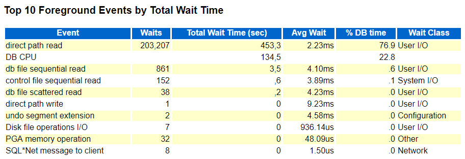

If I repeat exactly the same test (same settings, number of processes, size of objects etc.) using Shared Server architecture, this is what I get:
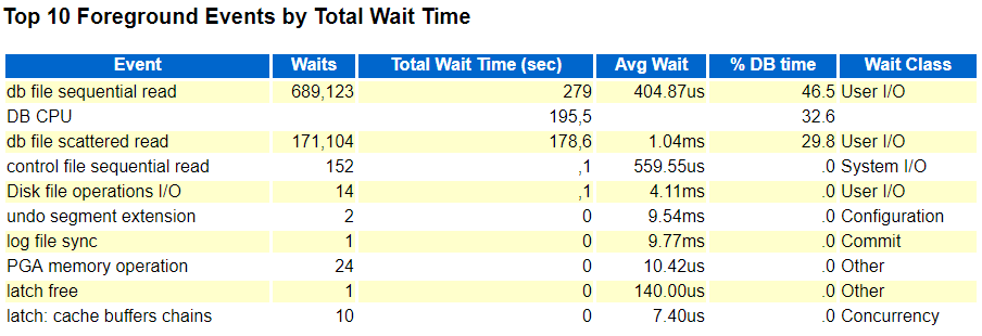
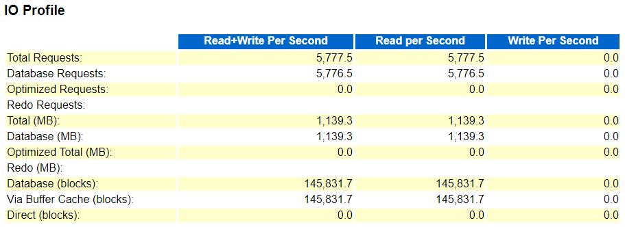
This is particularly interesting - no direct path reads although the benchmark sessions set in this case "_serial_direct_read" = 'always'.
In principle the same can be seen when running the maximum read IOPS benchmark, here is the expected result when using Dedicated Servers in asynchronous I/O mode:
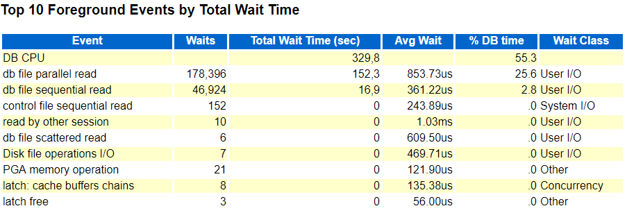
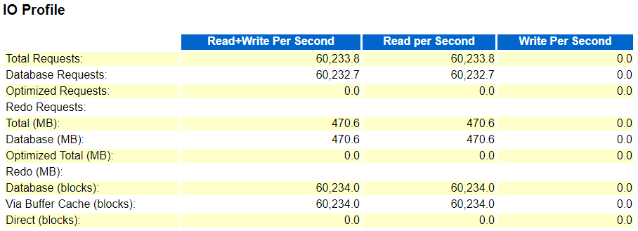
And again, this is what I get when running the same test using Shared Servers:

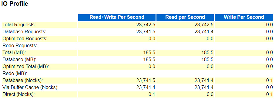
Again no sign of asynchronous I/O ("db file parallel read") - and the achieved IOPS rate is significantly lower, which is exactly what the client experienced, much more DB time waiting for I/O and less time spent on CPU than expected. Depending on the particular storage configuration and latency the difference when using the same number of processes can be even more significant, I've seen up to factor 20 difference in achieved IOPS rate, and factor 3 to 4 is quite typical. Of course as usual how relevant this really is all depends on the actual query, execution plan and data pattern and where most of the time is spent.
Also, it is important to point out that all this might not be too relevant to most configurations, since Shared Servers aren't used that much nowadays in the times of application servers / connection pools dominating typical environments. Also it's probably rather uncommon to use Shared Servers for batch processing tasks like this client did.
Although Shared Servers were originally designed for typical OLTP applications having many open sessions being idle most of the time and performing mostly very simple and straightforward operations (like looking up a few rows via an efficient index access path) it's still interesting to see this limitation that can be quite significant depending on the I/O patterns used. So far I've not seen this documented anywhere, also on MyOracleSupport I couldn't find any matching notes describing the behaviour, and unfortunately no Service Request was opened for the issue yet.
When using Parallel Execution, by the way, which is also very unlikely when using Shared Servers but perfectly possible (the Shared Server session then acts as Query Coordinator), the Parallel Servers can make use of asynchronous I/O - so the limitation only seems to apply to the Shared Server session itself. I can think of some reasons why this limitation could be explained from an implementation point of view the way Shared Servers work, but this is of course only speculation.
All currently relevant versions show the same behaviour in that regard, by the way. I've reproduced this on 11.2.0.4, 12.1.0.2 and 12.2.0.1 on Windows as well as on Linux.
Oracle Database Physical I/O IOPS And Throughput Benchmark
I've used a similar set of scripts quite a few times now to provide feedback to customers that wanted to get a more realistic picture of the I/O capabilities from a database perspective, rather than relying on artificial benchmarks performed outside - or even inside, think of I/O calibration - the database. Although there are already several Oracle benchmark toolkits available, like Swingbench and in particular SLOB, that run inside the database I was looking for a very simplistic and straightforward I/O benchmark that comes with minimum overhead and in principle allows maximizing I/O from the database perspective, so using regular Oracle database codepaths based on SQL execution plans, I/O calls performed as part of that, involving the database buffer cache where applicable and in particular supports focusing on specific I/O patterns (which might be unique to this benchmark toolkit). Therefore I've developed a set of simple scripts that support in total four different I/O tests:
- Single and multi block physical reads
- Single and multi block physical writes
In case of the physical read tests support for synchronous and asynchronous reads is provided, which can be controlled via a corresponding input / parameter to the script.
In terms of instrumentation / internal implementation this corresponds to:
- synchronous single block reads: "db file sequential read" / "cell single block physical read" on Exadata
- asynchronous single block reads: "db file parallel read" / "cell list of blocks physical read" on Exadata
- synchronous multi block reads: "db file scattered read" / "cell multiblock physical read" on Exadata
- asynchronous multi block reads: "direct path read" / "cell smart table/index scan" on Exadata
The physical write tests should mainly trigger "db file parallel write" in case of the single block writes and "direct path write" in case of the multi block writes. Of course when it comes to DML activity things get more complicated in terms of the actual database activity triggered, in particular the additional undo / redo / archiving / potential standby activity. Note that if you're using an auto-extensible Undo tablespace configuration, running the single block physical write tests might increase the size of your Undo tablespace - you have been warned.
So each I/O test generates a specific I/O pattern (except for the single block write test that can also trigger synchronous single block reads, see the script for more details). The basic idea is to run just one of the tests to maximize the specific I/O pattern, but of course nothing stops you from running several of the tests at the same time (would require different schemas to use for each test because otherwise object names dropped / created will collide / overlap) which will result in a mixture of I/O patterns. There is no synchronisation though in terms of starting / stopping / generating performance report snapshots etc. when running multiple of these tests at the same time, so you would probably have to take care of that yourself. So far I've not tested this, so it might not work out as just described.
In case of the physical read tests (except for the asynchronous "direct path read" that bypasses the buffer cache by definition) using too small objects / a too large buffer cache can turn this into a CPU / logical I/O test instead, so in principle you could use those tests for generating mainly CPU load instead of physical I/O (and provided the physical I/O is quick enough the CPU usage will be significant anyway), but that is not the intended usage of the scripts.
The scripts allow control over the size of the objects created and also support placing in specific buffer caches via the STORAGE clause (like RECYCLE or KEEP cache), so it is up to you to create objects of a suitable size depending on your configuration and intended usage.
Usage
Please note - the scripts are freely available and come with no warranty at all - so please use at your own risk.
In principle the scripts can be downloaded from my github repository - ideally pick the IO_BENCHMARK.ZIP which contains all required scripts, and should simply be extracted into some directory. Since the four different I/O tests are so similar, there is a subdirectory "common" under "io_benchmark" that holds all the common script parts and the main scripts then just call these common scripts where applicable.
The benchmark scripts consist of four similar sets:
max_read_iops_benchmark*: Single block reads synchronous / asynchronous
max_read_throughput_benchmark*: Multi block reads synchronous / asynchronous
max_write_iops_benchmark*: Single block writes - optionally mixed with synchronous single block reads (depends on object vs. buffer cache size)
max_write_throughput_benchmark*: Multi block direct writes
Each set consists of three scripts - an interactive guided script prompting for inputs used as parameters for the actual benchmark harness that in turn will launch another "slave" script as many times as desired to run the concurrent benchmark code.
There are in principle two different ways how the scripts can be used:
1. For each set there is a script that is supposed to be used from a SYSDBA account and guides through the different options available (*interactive). It will drop and re-create a schema to be used for the benchmark and grant the minimum privileges required to create the objects and run the benchmark. At the end of this interactive script it will connect as the user just created and run the benchmark. You can also use this script to clean-up afterwards, which is dropping the user created and stopping the script at that point.
2. The interactive script just calls the main benchmark harness with the parameters specified, so if you already have everything in place (check the "interactive_create_user.sql" in the "common" script subdirectory for details what privileges are required) to run the benchmark you can simply connect as the intended user, call the actual benchmark script and specify the parameters as desired - it will use defaults for any parameter not explicitly specified - check the script header for more details. Please note that I haven't tested running the actual benchmark as SYS respectively SYSDBA and I wouldn't recommend doing so. Instead use a dedicated user / schema as created by the interactive script part.
Each set of scripts consists of a third script which is the "slave" script being called as many times concurrently as specified to perform the actual benchmark activity.
The scripts will generate objects, typically as part of the preparation steps before the actual concurrent benchmark activity starts, or in case of the multi block write test, the object creation is the actual benchmark activity.
After the benchmark ran for the specified amount of time (600 seconds / 10 minutes default) the "slaves" will be shut down (if they haven't done so automatically) and the corresponding information about the IOPS / throughput rate achieved will be shown, based on (G)V$SYSMETRIC_HISTORY, so at least 120 seconds of runtime are required to have this final query to show something meaningful (to ensure that at least one 60 seconds interval is fully covered).
In addition the script by default will generate performance report snapshots (either AWR or STATSPACK) and display the corresponding report at the end. The file name generated describes the test performed along with the most important parameters (parallel degree, I/O mode (sync / async), object size, duration, timestamp etc.) Note that the script on Unix/Linux makes use of the "xdg-open" utility to open the generated report, so the "xdg-utils" package would be required to be installed to have this working as intended.
Note that in 12.2.0.1 the PDB level reports and metrics seem to miss "physical single block writes" performed by the DB Writer, so effectively evaluating / running this benchmark in 12.2.0.1 on PDB level won't report anything meaningful - you would have to resort to reports on CDB level instead, which I haven't implemented (actually I had to put in some effort to use the PDB level AWR reports and metrics in 12.2, so hopefully Oracle will fix this in future versions).
Finally the benchmark script will clean up and drop the objects created for the benchmark.
In principle the benchmark scripts should cope with all kinds of configurations: Windows / Unix / Linux, Single Instance / RAC, Standard / Enterprise Edition, PDB / Non-PDB, Non-Exadata / Exadata, and support versions from 11.2.0.4 on. It might run on lower versions, too, but not tested, and of course 18c (12.2.0.2) is not available on premises yet at the time of writing this, so not tested either.
But since this is 1.0 version it obviously wasn't tested in all possible combinations / configurations / parameter settings, so expect some glitches. Feedback and ideas how to improve are welcome.
Where applicable the benchmark harness script also generates two tables EVENT_HISTOGRAM_MICRO1 and EVENT_HISTOGRAM_MICRO2 which are snapshots of GV$EVENT_HISTOGRAM_MICRO available from 12.1 on for synchronous single / multi block reads. The "harness" scripts provide a suitable query in the script header to display the latency histogram information nicely.
Happy I/O benchmarking!
DOAG 2017 and IT Tage 2017 Presentation Material
You can find the slide deck here at slideshare.net.
Stay tuned for more publications this year - at least I have some interesting stuff upcoming.
DOAG Red Stack Magazin Artikelreihe "Oracle Database Cloud Performance" (German)
Die Artikelserie basiert auf den hier bereits publizierten Erkenntnissen in diesem Bereich und führt diese weiter fort.
Der erste Teil geht auf die verschiedenen Aspekte der maximal erreichbare Performance ein (CPU, Storage etc.), der zweite Teil wird in der nächsten Ausgabe zu lesen sein und legt den Schwerpunkt auf die Konsistenz der Performance, also wie konsistent sich die Datenbanken in der Cloud in Bezug auf Performance während der Tests verhalten haben.
New workshop "Exadata For Developers"
It covers in detail Smart Scans, the Exadata Flash Cache, Hybrid Columnar Compression and all surrounding features like Storage Indexes, (serial) direct path reads etc. etc.. Of course it also includes features that were added in 12c, like Attribute Clustering and Zone Maps.
All features are presented with live demo scripts, and there will be enough time to discuss your specific questions and analyse existing applications if desired.
For more information and details, check the corresponding pages:
German: Exadata für Anwendungsentwickler
English: Exadata For Developers
Oracle Database Cloud (DBaaS) Performance - Part 4 - Network
I've used the freely available "iperf" tool to measure the network bandwidth and got the following results:
[root@test12102rac2 ~]# iperf3 -c 10.196.49.126
Connecting to host 10.196.49.126, port 5201
[ 4] local 10.196.49.130 port 41647 connected to 10.196.49.126 port 5201
[ ID] Interval Transfer Bandwidth Retr Cwnd
[ 4] 0.00-1.00 sec 651 MBytes 5.46 Gbits/sec 15 786 KBytes
[ 4] 1.00-2.00 sec 823 MBytes 6.90 Gbits/sec 11 1.07 MBytes
[ 4] 2.00-3.00 sec 789 MBytes 6.62 Gbits/sec 7 1014 KBytes
[ 4] 3.00-4.00 sec 700 MBytes 5.87 Gbits/sec 39 1.04 MBytes
[ 4] 4.00-5.00 sec 820 MBytes 6.88 Gbits/sec 21 909 KBytes
[ 4] 5.00-6.00 sec 818 MBytes 6.86 Gbits/sec 17 1.17 MBytes
[ 4] 6.00-7.00 sec 827 MBytes 6.94 Gbits/sec 21 1005 KBytes
[ 4] 7.00-8.00 sec 792 MBytes 6.64 Gbits/sec 8 961 KBytes
[ 4] 8.00-9.00 sec 767 MBytes 6.44 Gbits/sec 4 1.11 MBytes
[ 4] 9.00-10.00 sec 823 MBytes 6.91 Gbits/sec 6 1.12 MBytes
- - - - - - - - - - - - - - - - - - - - - - - - -
[ ID] Interval Transfer Bandwidth Retr
[ 4] 0.00-10.00 sec 7.63 GBytes 6.55 Gbits/sec 149 sender
[ 4] 0.00-10.00 sec 7.63 GBytes 6.55 Gbits/sec receiver
iperf Done.
For completeness, the UDP results look like the following:
[root@test12102rac2 ~]# iperf3 -c 10.196.49.126 -u -b 10000M
Connecting to host 10.196.49.126, port 5201
[ 4] local 10.196.49.130 port 55482 connected to 10.196.49.126 port 5201
[ ID] Interval Transfer Bandwidth Total Datagrams
[ 4] 0.00-1.00 sec 494 MBytes 4.14 Gbits/sec 63199
[ 4] 1.00-2.00 sec 500 MBytes 4.20 Gbits/sec 64057
[ 4] 2.00-3.00 sec 462 MBytes 3.87 Gbits/sec 59102
[ 4] 3.00-4.00 sec 496 MBytes 4.16 Gbits/sec 63491
[ 4] 4.00-5.00 sec 482 MBytes 4.05 Gbits/sec 61760
[ 4] 5.00-6.00 sec 425 MBytes 3.57 Gbits/sec 54411
[ 4] 6.00-7.00 sec 489 MBytes 4.10 Gbits/sec 62574
[ 4] 7.00-8.00 sec 411 MBytes 3.45 Gbits/sec 52599
[ 4] 8.00-9.00 sec 442 MBytes 3.71 Gbits/sec 56541
[ 4] 9.00-10.00 sec 481 MBytes 4.04 Gbits/sec 61614
- - - - - - - - - - - - - - - - - - - - - - - - -
[ ID] Interval Transfer Bandwidth Jitter Lost/Total Datagrams
[ 4] 0.00-10.00 sec 4.57 GBytes 3.93 Gbits/sec 0.028 ms 23434/599340 (3.9%)
[ 4] Sent 599340 datagrams
iperf Done.
[Update 6.2.2017]: Thanks to Frits Hoogland who pointed out the very high "max" value for the ping. Although I didn't spot the pattern that he saw in a different network test setup ("cross cloud platform"), which was an initial slowness, it's still worth to point out the high "max" value of almost 200 ms for a ping, and also the "mdev" value of 3.322 ms seems to suggest that there were some significant variations in ping times observed that are potentially hidden behind the average values provided. I'll repeat the ping test and see if I can reproduce these outliers and if yes, find out more details.